The content of this blog is based on some exploratory data analysis performed on the corpora provided for the “Spooky Author Identification” challenge at Kaggle [1]. The corpora includes excerpts/ sentences from some of the scariest writer of all times.

The Spooky Challenge
An Hallowen-based challenge [1] with the following goal: predict who was writing a sentence of a possible spooky story between Edgar Allan Poe, HP Lovecraft and Mary Wollstonecraft Shelley.
“Deep into that darkness peering, long I stood there, wondering, fearing, doubting, dreaming dreams no mortal ever dared to dream before.” Edgar Allan Poe
“That is not dead which can eternal lie, And with strange aeons even death may die.” HP Lovecraft
“Life and death appeared to me ideal bounds, which I should first break through, and pour a torrent of light into our dark world.” Mary Wollstonecraft Shelley
The Toolset
The only tools available to us during this exploration will be our intuition, curiosity and the selected packages. Specifically:
tidytextpackage, text mining for word processing and sentiment analysis using tidy toolstidyversepackage, an opinionated collection of R packages designed for data sciencewordcloudpackage, pretty word cloudsgridExtrapackage, supporting functions to work withgridgraphicscaretpackage, supporting function for performing stratified random samplingcorrplotpackage, a graphical display of a correlation matrix, confidence interval
# Required libraries
# if packages not installed
#install.packages("packageName")

library(tidytext)
library(tidyverse)
library(gridExtra)
library(wordcloud)
library(dplyr)
library(corrplot)
The Beginning of the Journey: the Spooky Data
We are given a csv file, the train.csv, containing some information about the authors. The information consists on a set of sentences written by the different authors (EAP, HPL, MWS). Each entry (line) in the file is an observation providing the following information:
- an
id, a unique id for the excerpt/ sentence (as a string) - the
text, the excerpt/ sentence (as a string), - the
author, the author of the excerpt/ sentence (as a string)- a categorical feature that can assume three possible values
EAPfor Edgar Allan Poe,HPLfor HP Lovecraft,MWSfor Mary Wollstonecraft Shelley
- a categorical feature that can assume three possible values
# loading the data using readr package
spooky_data <- readr::read_csv(file = "./../../../data/train.csv",
                              col_types = "ccc",
                              locale = locale("en"),
                              na = c("", "NA"))

# readr::read_csv does not transform string into factor
# being the author feature categorical by nature
# it is transformed into a factor
spooky_data$author <- as.factor(spooky_data$author)
The overall data includes 19579 observations with 3 features (id, text, author). Specifically 7900 excerpts (40.35 %) of Edgard Allan Poe, 5635 excerpts (28.78 %) of HP Lovecraft and 6044 excerpts (30.87 %) of Mary Wollstonecraft Shelley.
Avoid the madness!
It is forbidden to use all of the provided spooky data for finding our way through the unique spookyness of each author. We still want to evaluate how our intuition generalizes on a unseen excerpt/ sentence, right?? For this reason the given training data is split in two parts (using stratified random sampling)
- an actual training dataset (70% of the excerpts/ sentences), used for
- exploration and insight creation, and
- traing the classification model
- a test dataset (the remaining 30% of the excerpts/ sentences), used for
- evaluation of the accuracy of our classification model.
# setting the seed for reproducibility
set.seed(19711004)
trainIndex <- caret::createDataPartition(spooky_data$author, p = 0.7, list = FALSE, times = 1)
spooky_training <- spooky_data[trainIndex,]
spooky_testing <- spooky_data[-trainIndex,]
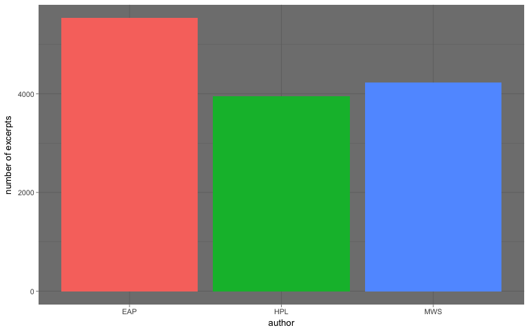
Specifically 5530 excerpts (40.35 %) of Edgard Allan Poe, 3945 excerpts (28.78 %) of HP Lovecraft and 4231 excerpts (30.87 %) of Mary Wollstonecraft Shelley.
Moving our first steps: from darkness into the light
Before start building any model, we need to understand tha data, build intuitions about the information contanined in the data and identify a way to use those intuitions to build a great predicting model.
Is the provided data useable?
Question: Does each observation has an id? An excerpt/ sentence associated to it? An author?
missingValueSummary <- colSums(is.na(spooky_training))
As we can see from the table below, there are no missing values in the dataset.
| id | text | author |
|---|---|---|
| 0 | 0 | 0 |
Some initial facts about the excerpts/ sentences
Below we can see, as an example, some of the observations (and excerpt/ sentence) available in our dataset
| id | text | author |
|---|---|---|
| id26305 | This process, however, afforded me no means of ascertaining the dimensions of my dungeon; as I might make its circuit, and return to the point whence I set out, without being aware of the fact; so perfectly uniform seemed the wall. | EAP |
| id22965 | A youth passed in solitude, my best years spent under your gentle and feminine fosterage, has so refined the groundwork of my character that I cannot overcome an intense distaste to the usual brutality exercised on board ship: I have never believed it to be necessary, and when I heard of a mariner equally noted for his kindliness of heart and the respect and obedience paid to him by his crew, I felt myself peculiarly fortunate in being able to secure his services. | MWS |
| id19764 | Herbert West needed fresh bodies because his life work was the reanimation of the dead. | HPL |
| id10125 | For many prodigies and signs had taken place, and far and wide, over sea and land, the black wings of the Pestilence were spread abroad. | EAP |
Question: How many excerpts/ sentences are available by author?
no_excerpts_by_author <- spooky_training %>%
  dplyr::group_by(author) %>%
  dplyr::summarise(n = n())

ggplot(data = no_excerpts_by_author,
              mapping = aes(x = author, y = n, fill = author)) +
         geom_col(show.legend = F) +
         ylab(label = "number of excerpts") +
         theme_dark(base_size = 10)
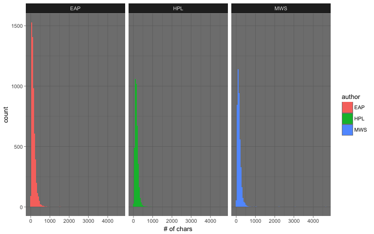
Question: How long (# ofchars) are the excerpts/ sentences by author?
spooky_training$len <- nchar(spooky_training$text)
ggplot(data = spooky_training, mapping = aes(x = len, fill = author)) +
  geom_histogram(binwidth = 50) +
  facet_grid(. ~ author) +
  xlab("# of chars") +
  theme_dark(base_size = 10)
ggplot(data = spooky_training, mapping = aes(x = 1, y = len)) +
  geom_boxplot(outlier.colour = "red", outlier.shape = 1) +
  facet_grid(. ~ author) +
  xlab(NULL) +
  ylab("# of chars") +
  theme_dark(base_size = 10)
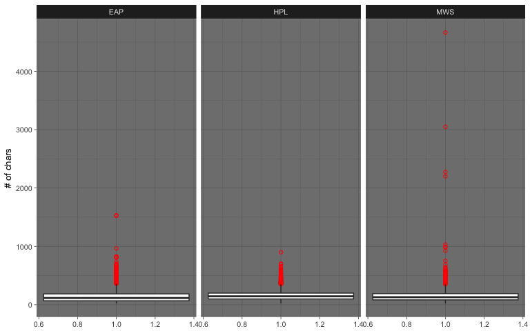
There are some excerpts that are very long. As we can see from the boxplot above, there are few outliers for each authors; a possible explanation is that the sentence segmentation had few hiccups (see deatils below).
| Author | Min (# chars) | Mean (# chars) | Median (# chars) | Max (# chars) |
|---|---|---|---|---|
| EAP | 21 | 141.92 | 115 | 1533 |
| HPL | 21 | 157.61 | 144 | 900 |
| MWS | 21 | 150.5 | 129 | 4663 |
For example Mary Wollstonecraft Shelley (MWS) has an excerpts of around 4600 characters:
“Diotima approached the fountain seated herself on a mossy mound near it and her disciples placed themselves on the grass near her Without noticing me who sat close under her she continued her discourse addressing as it happened one or other of her listeners but before I attempt to repeat her words I will describe the chief of these whom she appeared to wish principally to impress One was a woman of about years of age in the full enjoyment of the most exquisite beauty her golden hair floated in ringlets on her shoulders her hazle eyes were shaded by heavy lids and her mouth the lips apart seemed to breathe sensibility But she appeared thoughtful unhappy her cheek was pale she seemed as if accustomed to suffer and as if the lessons she now heard were the only words of wisdom to which she had ever listened The youth beside her had a far different aspect his form was emaciated nearly to a shadow his features were handsome but thin worn his eyes glistened as if animating the visage of decay his forehead was expansive but there was a doubt perplexity in his looks that seemed to say that although he had sought wisdom he had got entangled in some mysterious mazes from which he in vain endeavoured to extricate himself As Diotima spoke his colour went came with quick changes the flexible muscles of his countenance shewed every impression that his mind received he seemed one who in life had studied hard but whose feeble frame sunk beneath the weight of the mere exertion of life the spark of intelligence burned with uncommon strength within him but that of life seemed ever on the eve of fading At present I shall not describe any other of this groupe but with deep attention try to recall in my memory some of the words of Diotima they were words of fire but their path is faintly marked on my recollection It requires a just hand, said she continuing her discourse, to weigh divide the good from evil On the earth they are inextricably entangled and if you would cast away what there appears an evil a multitude of beneficial causes or effects cling to it mock your labour When I was on earth and have walked in a solitary country during the silence of night have beheld the multitude of stars, the soft radiance of the moon reflected on the sea, which was studded by lovely islands When I have felt the soft breeze steal across my cheek as the words of love it has soothed cherished me then my mind seemed almost to quit the body that confined it to the earth with a quick mental sense to mingle with the scene that I hardly saw I felt Then I have exclaimed, oh world how beautiful thou art Oh brightest universe behold thy worshiper spirit of beauty of sympathy which pervades all things, now lifts my soul as with wings, how have you animated the light the breezes Deep inexplicable spirit give me words to express my adoration; my mind is hurried away but with language I cannot tell how I feel thy loveliness Silence or the song of the nightingale the momentary apparition of some bird that flies quietly past all seems animated with thee more than all the deep sky studded with worlds" If the winds roared tore the sea and the dreadful lightnings seemed falling around me still love was mingled with the sacred terror I felt; the majesty of loveliness was deeply impressed on me So also I have felt when I have seen a lovely countenance or heard solemn music or the eloquence of divine wisdom flowing from the lips of one of its worshippers a lovely animal or even the graceful undulations of trees inanimate objects have excited in me the same deep feeling of love beauty; a feeling which while it made me alive eager to seek the cause animator of the scene, yet satisfied me by its very depth as if I had already found the solution to my enquires sic as if in feeling myself a part of the great whole I had found the truth secret of the universe But when retired in my cell I have studied contemplated the various motions and actions in the world the weight of evil has confounded me If I thought of the creation I saw an eternal chain of evil linked one to the other from the great whale who in the sea swallows destroys multitudes the smaller fish that live on him also torment him to madness to the cat whose pleasure it is to torment her prey I saw the whole creation filled with pain each creature seems to exist through the misery of another death havoc is the watchword of the animated world And Man also even in Athens the most civilized spot on the earth what a multitude of mean passions envy, malice a restless desire to depreciate all that was great and good did I see And in the dominions of the great being I saw man reduced?”
Thinking Point: “What do we want to do with those excerpts/ outliers?”.
Some more facts about the excerpts/ sentences using the bag-of-words
The data is transformed into a tidy format (unigrams only) in order to use the tidy tools to perform some basic and essential NLP operations.
spooky_trainining_tidy_1n <- spooky_training %>%
  select(id, text, author) %>%
  tidytext::unnest_tokens(output = word,
                          input = text,
                          token = "words",
                          to_lower = TRUE)
Each sentence is tokenised into words (normalised to lower case, removed punctuation). See example below how the data (each excerpt/ sentence) was and how it has been transformed
| id | text | author |
|---|---|---|
| id17189 | But a glance will show the fallacy of this idea. | EAP |
| id | author | word |
|---|---|---|
| id17189 | EAP | but |
| id17189 | EAP | a |
| id17189 | EAP | glance |
| id17189 | EAP | will |
| id17189 | EAP | show |
| id17189 | EAP | the |
| id17189 | EAP | fallacy |
| id17189 | EAP | of |
| id17189 | EAP | this |
| id17189 | EAP | idea |
Question: Which are the most common words used by each author?
Lets start to count how many times words has been used by each author and plot …
words_author_1 <- plot_common_words_by_author(x = spooky_trainining_tidy_1n,
                                         author = "EAP",
                                         greater.than = 500)

words_author_2 <- plot_common_words_by_author(x = spooky_trainining_tidy_1n,
                                         author = "HPL",
                                         greater.than = 500)
words_author_3 <- plot_common_words_by_author(x = spooky_trainining_tidy_1n,
                                         author = "MWS",
                                         greater.than = 500)

gridExtra::grid.arrange(words_author_1, words_author_2, words_author_3, nrow = 1)
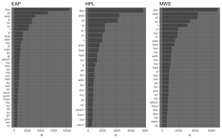
From this initial visualization we can see that the authors use quite often the same set of words - like the, and, of. These words do not give any actual information about the vocabulary actually used by each author, they are common words that represent just noise when working with unigrams: they are usually called stopwords.
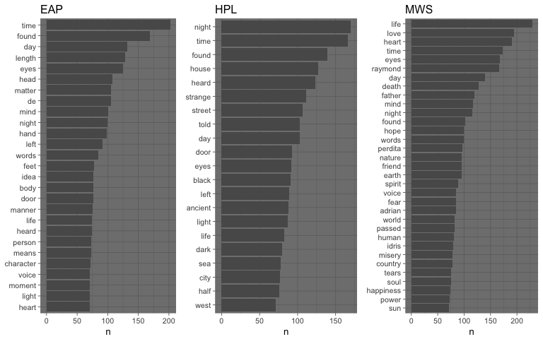
If the stopwords are removed, using the list of stopwords provided by the tidytext package, it is possible to see that the authors do actually used different words more frequently than others (and it differs from author to author, the author vocabulary footprint).
words_author_1 <- plot_common_words_by_author(x = spooky_trainining_tidy_1n,
                                         author = "EAP",
                                         greater.than = 70,
                                         remove.stopwords = T)

words_author_2 <- plot_common_words_by_author(x = spooky_trainining_tidy_1n,
                                         author = "HPL",
                                         greater.than = 70,
                                         remove.stopwords = T)

words_author_3 <- plot_common_words_by_author(x = spooky_trainining_tidy_1n,
                                         author = "MWS",
                                         greater.than = 70,
                                         remove.stopwords = T)

gridExtra::grid.arrange(words_author_1, words_author_2, words_author_3, nrow = 1)
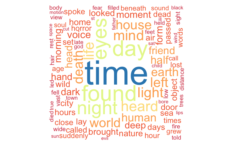
Another way to visualize the most frequent words by author is to use wordclouds. Wordclouds make it easy to spot differences, the importance of each word matches its font size and color.
par(mfrow = c(1,3), mar = c(0,0,0,0))

words_author <- get_common_words_by_author(x = spooky_trainining_tidy_1n,
                           author = "EAP",
                           remove.stopwords = TRUE)

mypal <- brewer.pal(8,"Spectral")
wordcloud(words = c("EAP", words_author$word),
          freq = c(max(words_author$n) + 100, words_author$n),
          colors = mypal,
          scale=c(7,.5),
          rot.per=.15,
          max.words = 100,
          random.order = F)

words_author <- get_common_words_by_author(x = spooky_trainining_tidy_1n,
                           author = "HPL",
                           remove.stopwords = TRUE)

mypal <- brewer.pal(8,"Spectral")
wordcloud(words = c("HPL", words_author$word),
          freq = c(max(words_author$n) + 100, words_author$n),
          colors = mypal,
          scale=c(7,.5),
          rot.per=.15,
          max.words = 100,
          random.order = F)

words_author <- get_common_words_by_author(x = spooky_trainining_tidy_1n,
                           author = "MWS",
                           remove.stopwords = TRUE)

mypal <- brewer.pal(8,"Spectral")
wordcloud(words = c("MWS", words_author$word),
          freq = c(max(words_author$n) + 100, words_author$n),
          colors = mypal,
          scale=c(7,.5),
          rot.per=.15,
          max.words = 100,
          random.order = F)
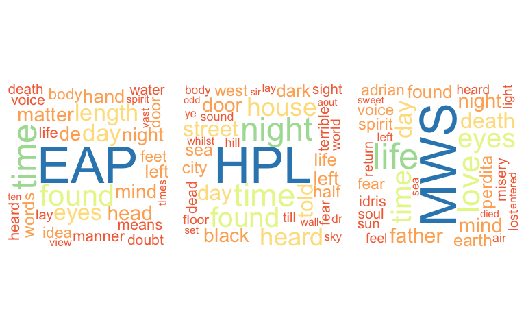
From the wordclouds we can infer that
EAPloves to use the wordstime,found,eyes,length,day, etc.HPLloves to use the wordsnight,time,found,house, etc.MWSloves to use the wordslife,time,love,eyesetc.
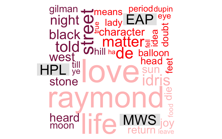
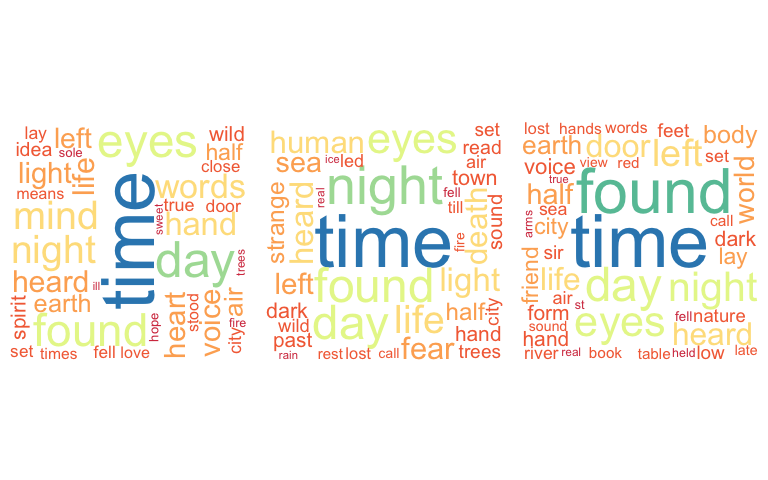
A comparison cloud can be used to compare the different authors. From the R documentation
‘Let p{i,j} be the rate at which word i occurs in document j, and p_j be the average across documents(∑ip{i,j}/ndocs). The size of each word is mapped to its maximum deviation ( max_i(p_{i,j}-p_j) ), and its angular position is determined by the document where that maximum occurs.’_
See below the comparison cloud between all authors…
comparison_data <- spooky_trainining_tidy_1n %>%
  dplyr::select(author, word) %>%
  dplyr::anti_join(stop_words) %>%
  dplyr::count(author,word, sort = TRUE)


comparison_data %>%
  reshape2::acast(word ~ author, value.var = "n", fill = 0) %>%
  comparison.cloud(colors = c("red", "violetred4", "rosybrown1"),
                   random.order = F,
                   scale=c(7,.5),
                   rot.per = .15,
                   max.words = 200)
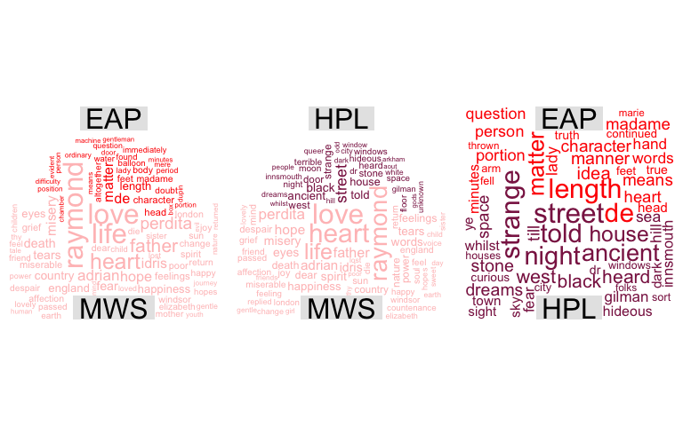
See below the comparison clouds between the authors, two authors at any time …
par(mfrow = c(1,3), mar = c(0,0,0,0))

comparison_EAP_MWS <- comparison_data %>%
  dplyr::filter(author == "EAP" | author == "MWS")

comparison_EAP_MWS %>%
  reshape2::acast(word ~ author, value.var = "n", fill = 0) %>%
  comparison.cloud(colors = c("red", "rosybrown1"),
                   random.order = F,
                   scale=c(3,.2),
                   rot.per = .15,
                   max.words = 100)

comparison_HPL_MWS <- comparison_data %>%
  dplyr::filter(author == "HPL" | author == "MWS")

comparison_HPL_MWS %>%
  reshape2::acast(word ~ author, value.var = "n", fill = 0) %>%
  comparison.cloud(colors = c("violetred4", "rosybrown1"),
                   random.order = F,
                   scale=c(3,.2),
                   rot.per = .15,
                   max.words = 100)


comparison_EAP_HPL <- comparison_data %>%
  dplyr::filter(author == "EAP" | author == "HPL")

comparison_EAP_HPL %>%
  reshape2::acast(word ~ author, value.var = "n", fill = 0) %>%
  comparison.cloud(colors = c("red", "violetred4"),
                   random.order = F,
                   scale=c(3,.2),
                   rot.per = .15,
                   max.words = 100)
Question: How many unique words are needed in the author dictionary to cover 90% of the used word instances?
words_cov_author_1 <- plot_word_cov_by_author(x = spooky_trainining_tidy_1n, author = "EAP")
words_cov_author_2 <- plot_word_cov_by_author(x = spooky_trainining_tidy_1n, author = "HPL")
words_cov_author_3 <- plot_word_cov_by_author(x = spooky_trainining_tidy_1n, author = "MWS")

gridExtra::grid.arrange(words_cov_author_1, words_cov_author_2, words_cov_author_3, nrow = 1)
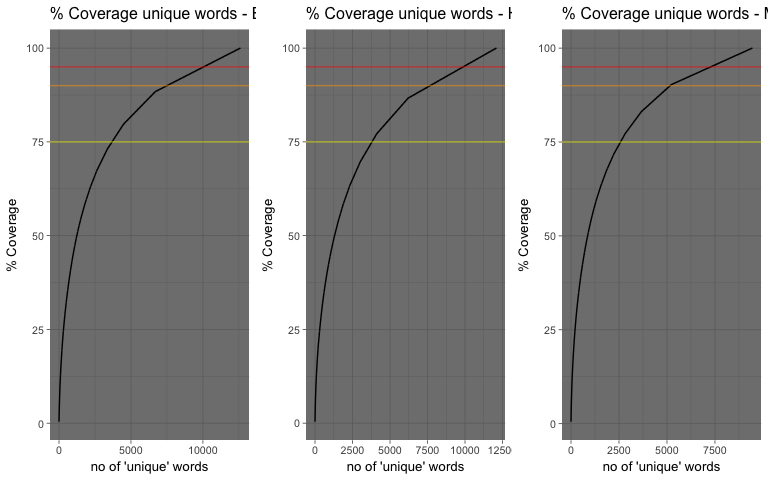
From the plot above we can see that for EAP and HPL provided corpus, we need circa 7500 words to cover 90% of word instance. While for MWS provided corpus, circa 5000 words are needed to cover 90% of word instances.
Question: Is there any commonality between the dictionaries used by the authors?
Are the authors using the same words? A commonality cloud can be used to answer this specific question, it emphasises the similarities between authors and plot a cloud showing the common words between the different authors. It shows only those words that are used by all authors with their combined frequency across authors.
See below the commonality cloud between all authors…
comparison_data <- spooky_trainining_tidy_1n %>%
  dplyr::select(author, word) %>%
  dplyr::anti_join(stop_words) %>%
  dplyr::count(author,word, sort = TRUE)

mypal <- brewer.pal(8,"Spectral")
comparison_data %>%
  reshape2::acast(word ~ author, value.var = "n", fill = 0) %>%
  commonality.cloud(colors = mypal,
                   random.order = F,
                   scale=c(7,.5),
                   rot.per = .15,
                   max.words = 200)
See below the commonality clouds between the authors, two authors at any time …
par(mfrow = c(1,3), mar = c(0,0,0,0))
mypal <- brewer.pal(8,"Spectral")

comparison_EAP_MWS <- comparison_data %>%
  dplyr::filter(author == "EAP" | author == "MWS")

comparison_EAP_MWS %>%
  reshape2::acast(word ~ author, value.var = "n", fill = 0) %>%
  commonality.cloud(colors = mypal,
                   random.order = F,
                   scale=c(7,.5),
                   rot.per = .15,
                   max.words = 200)

comparison_HPL_MWS <- comparison_data %>%
  dplyr::filter(author == "HPL" | author == "MWS")

comparison_HPL_MWS %>%
  reshape2::acast(word ~ author, value.var = "n", fill = 0) %>%
  commonality.cloud(colors = mypal,
                   random.order = F,
                   scale=c(7,.5),
                   rot.per = .15,
                   max.words = 200)

comparison_EAP_HPL <- comparison_data %>%
  dplyr::filter(author == "EAP" | author == "HPL")

comparison_EAP_HPL %>%
  reshape2::acast(word ~ author, value.var = "n", fill = 0) %>%
  commonality.cloud(colors = mypal,
                   random.order = F,
                   scale=c(7,.5),
                   rot.per = .15,
                   max.words = 200)
Question: Can Word Frequencies be used to compare different authors?
First of all we need to prepare the data calculating the word frequencies for each author …
word_freqs <- spooky_trainining_tidy_1n %>%
  dplyr::anti_join(stop_words) %>%
  dplyr::count(author, word) %>%
  dplyr::group_by(author) %>%
  dplyr::mutate(word_freq = n/ sum(n)) %>%
  dplyr::select(-n)
| author | word | word_freq |
|---|---|---|
| EAP | à | 0.0001179 |
| EAP | a.m | 0.0000589 |
| EAP | ab | 0.0000196 |
| EAP | aback | 0.0000393 |
| EAP | abandon | 0.0001179 |
then we need to spread the author (key) and the word frequency (value) across multiple columns (note how NAs have been introduced for word not used by an author) …
word_freqs <- word_freqs%>%
  tidyr::spread(author, word_freq)
| word | EAP | HPL | MWS |
|---|---|---|---|
| à | 0.0001179 | NA | NA |
| a.d | NA | 0.0000454 | NA |
| a.m | 0.0000589 | 0.0001362 | NA |
| ab | 0.0000196 | NA | NA |
| aback | 0.0000393 | NA | NA |
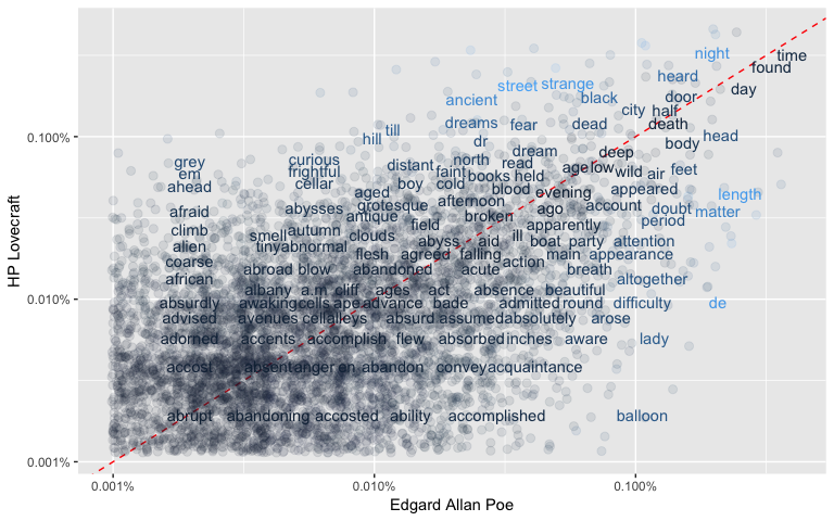
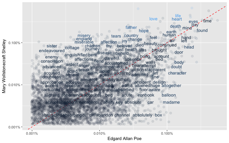
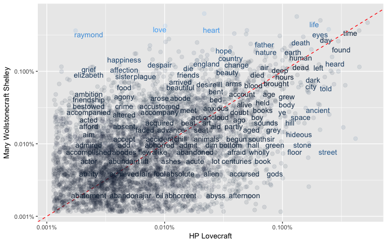
Lets start to plot the word frequencies (log scale) comparing two authors at a time and see how words distribute on the plane. Words that are close to the line (y = x) have similar frequencies in both sets of texts. While words that are far from the line are words that are found more in one set of texts than another.
As we can see in the plots below - there are some words close to the line but most of the words are around the line showing a difference between the frequencies.
# Removing incomplete cases - not all words are common for the authors
# when spreading words to all authors - some will get NAs (if not used
# by an author)

word_freqs_EAP_vs_HPL <- word_freqs %>%
  dplyr::select(word, EAP, HPL) %>%
  dplyr::filter(!is.na(EAP) & !is.na(HPL))

ggplot(data = word_freqs_EAP_vs_HPL, mapping = aes(x = EAP, y = HPL, color = abs(EAP - HPL))) +
  geom_abline(color = "red", lty = 2) +
  geom_jitter(alpha = 0.1, size = 2.5, width = 0.3, height = 0.3) +
  geom_text(aes(label = word), check_overlap = TRUE, vjust = 1.5) +
  scale_x_log10(labels = scales::percent_format()) +
  scale_y_log10(labels = scales::percent_format()) +
  theme(legend.position = "none") +
  labs(y = "HP Lovecraft", x = "Edgard Allan Poe")
# Removing incomplete cases - not all words are common for the authors
# when spreading words to all authors - some will get NAs (if not used
# by an author)

word_freqs_EAP_vs_MWS <- word_freqs %>%
  dplyr::select(word, EAP, MWS) %>%
  dplyr::filter(!is.na(EAP) & !is.na(MWS))

ggplot(data = word_freqs_EAP_vs_MWS, mapping = aes(x = EAP, y = MWS, color = abs(EAP - MWS))) +
  geom_abline(color = "red", lty = 2) +
  geom_jitter(alpha = 0.1, size = 2.5, width = 0.3, height = 0.3) +
  geom_text(aes(label = word), check_overlap = TRUE, vjust = 1.5) +
  scale_x_log10(labels = scales::percent_format()) +
  scale_y_log10(labels = scales::percent_format()) +
  theme(legend.position = "none") +
  labs(y = "Mary Wollstonecraft Shelley", x = "Edgard Allan Poe")
# Removing incomplete cases - not all words are common for the authors
# when spreading words to all authors - some will get NAs (if not used
# by an author)
word_freqs_HPL_vs_MWS <- word_freqs %>%
  dplyr::select(word, HPL, MWS) %>%
  dplyr::filter(!is.na(HPL) & !is.na(MWS))

ggplot(data = word_freqs_HPL_vs_MWS, mapping = aes(x = HPL, y = MWS, color = abs(HPL - MWS))) +
  geom_abline(color = "red", lty = 2) +
  geom_jitter(alpha = 0.1, size = 2.5, width = 0.3, height = 0.3) +
  geom_text(aes(label = word), check_overlap = TRUE, vjust = 1.5) +
  scale_x_log10(labels = scales::percent_format()) +
  scale_y_log10(labels = scales::percent_format()) +
  theme(legend.position = "none") +
  labs(y = "Mary Wollstonecraft Shelley", x = "HP Lovecraft")
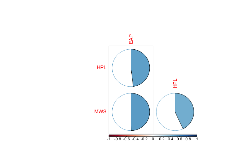
In order to quantify how similar/ different these sets of word frequencies by author, are we can calculate a correlation (Pearson for linearity) measurement between the sets. There is a correlation of around 0.48 to 0.5 between the different authors (see plot below).
word_freqs %>%
  select(-word) %>%
  cor(use="complete.obs", method="spearman") %>%
  corrplot(type="lower",
           method="pie",
           diag = F)
References
[1] Kaggle challenge: Spooky AUthor Identification
[2] “Text Mining in R - A tidy Approach” by J. Silge & D. Robinsons, O’Reilly 2017
[3] “Regular Expressions, Text Normalization and Edit Distance” draft chapter by D. Jurafsky & J. H . Martin, 2018
Appendix: Supporting functions
getNoExcerptsFor <- function(x, author){
  sum(x$author == author)
}

getPercentageExcerptsFor <- function(x, author){
  round((sum(x$author == author)/ dim(x)[1]) * 100, digits = 2)
}

get_xxx_length <- function(x, author, func){
  round(func(x[x$author == author,]$len), digits = 2)
}

plot_common_words_by_author <- function(x, author, remove.stopwords = FALSE, greater.than = 90){
  the_title = author
  if(remove.stopwords){
    x <- x %>% dplyr::anti_join(stop_words)
  }

  x[x$author == author,] %>%
    dplyr::count(word, sort = TRUE) %>%
    dplyr::filter(n > greater.than) %>%
    dplyr::mutate(word = reorder(word, n)) %>%
    ggplot(mapping = aes(x = word, y = n)) +
    geom_col() +
    xlab(NULL) +
    ggtitle(the_title) +
    coord_flip() +
    theme_dark(base_size = 10)
}

get_common_words_by_author <- function(x, author, remove.stopwords = FALSE){
  if(remove.stopwords){
    x <- x %>% dplyr::anti_join(stop_words)
  }

  x[x$author == author,] %>%
    dplyr::count(word, sort = TRUE)
}

plot_word_cov_by_author <- function(x,author){
  words_author <- get_common_words_by_author(x,
                                             author,
                                             remove.stopwords = TRUE)
  words_author %>%
    mutate(cumsum = cumsum(n),
           cumsum_perc = round(100 * cumsum/sum(n), digits = 2)) %>%
    ggplot(mapping = aes(x = 1:dim(words_author)[1], y = cumsum_perc)) +
    geom_line() +
    geom_hline(yintercept = 75, color = "yellow", alpha = 0.5) +
    geom_hline(yintercept = 90, color = "orange", alpha = 0.5) +
    geom_hline(yintercept = 95, color = "red", alpha = 0.5) +
    xlab("no of 'unique' words") +
    ylab("% Coverage") +
    ggtitle(paste("% Coverage unique words -", author, sep = " ")) +
    theme_dark(base_size = 10)
}
Session Info
sessionInfo()
## R version 3.3.3 (2017-03-06)
## Platform: x86_64-apple-darwin13.4.0 (64-bit)
## Running under: macOS  10.13
##
## locale:
## [1] no_NO.UTF-8/no_NO.UTF-8/no_NO.UTF-8/C/no_NO.UTF-8/no_NO.UTF-8
##
## attached base packages:
## [1] stats     graphics  grDevices utils     datasets  methods   base
##
## other attached packages:
##  [1] bindrcpp_0.2       corrplot_0.84      wordcloud_2.5
##  [4] RColorBrewer_1.1-2 gridExtra_2.3      dplyr_0.7.3
##  [7] purrr_0.2.3        readr_1.1.1        tidyr_0.7.1
## [10] tibble_1.3.4       ggplot2_2.2.1      tidyverse_1.1.1
## [13] tidytext_0.1.3
##
## loaded via a namespace (and not attached):
##  [1] httr_1.3.1         ddalpha_1.2.1      splines_3.3.3
##  [4] jsonlite_1.5       foreach_1.4.3      prodlim_1.6.1
##  [7] modelr_0.1.1       assertthat_0.2.0   highr_0.6
## [10] stats4_3.3.3       DRR_0.0.2          cellranger_1.1.0
## [13] yaml_2.1.14        robustbase_0.92-7  slam_0.1-40
## [16] ipred_0.9-6        backports_1.1.0    lattice_0.20-35
## [19] glue_1.1.1         digest_0.6.12      rvest_0.3.2
## [22] colorspace_1.3-2   recipes_0.1.0      htmltools_0.3.6
## [25] Matrix_1.2-11      plyr_1.8.4         psych_1.7.8
## [28] timeDate_3012.100  pkgconfig_2.0.1    CVST_0.2-1
## [31] broom_0.4.2        haven_1.1.0        caret_6.0-77
## [34] scales_0.5.0       gower_0.1.2        lava_1.5
## [37] withr_2.0.0        nnet_7.3-12        lazyeval_0.2.0
## [40] mnormt_1.5-5       survival_2.41-3    magrittr_1.5
## [43] readxl_1.0.0       evaluate_0.10.1    tokenizers_0.1.4
## [46] janeaustenr_0.1.5  nlme_3.1-131       SnowballC_0.5.1
## [49] MASS_7.3-47        forcats_0.2.0      xml2_1.1.1
## [52] dimRed_0.1.0       foreign_0.8-69     class_7.3-14
## [55] tools_3.3.3        hms_0.3            stringr_1.2.0
## [58] kernlab_0.9-25     munsell_0.4.3      RcppRoll_0.2.2
## [61] rlang_0.1.2        grid_3.3.3         iterators_1.0.8
## [64] labeling_0.3       rmarkdown_1.6      gtable_0.2.0
## [67] ModelMetrics_1.1.0 codetools_0.2-15   reshape2_1.4.2
## [70] R6_2.2.2           lubridate_1.6.0    knitr_1.17
## [73] bindr_0.1          rprojroot_1.2      stringi_1.1.5
## [76] parallel_3.3.3     Rcpp_0.12.12       rpart_4.1-11
## [79] tidyselect_0.2.0   DEoptimR_1.0-8