The content of this blog is based on some classification performed on the corpora provided for the “Spooky Author Identification” challenge at Kaggle [1]. An Hallowen-based challenge with the following goal: predict who was writing a sentence of a possible spooky story between Edgar Allan Poe, HP Lovecraft and Mary Wollstonecraft Shelley.
“Deep into that darkness peering, long I stood there, wondering, fearing, doubting, dreaming dreams no mortal ever dared to dream before.” Edgar Allan Poe
“That is not dead which can eternal lie, And with strange aeons even death may die.” HP Lovecraft
“Life and death appeared to me ideal bounds, which I should first break through, and pour a torrent of light into our dark world.” Mary Wollstonecraft Shelley
Naive Bayes classifiers are a family of simple probabilistic classifiers that can be used to perform text categorization , the task of classifying a text/ document with a label taken out from a set of (given) labels. Examples of text categorization tasks are:
- sentiment analysis, the extraction of sentiment from a sentence
- spam detection, determining if a message/ email is spam
- authorship attribution, determining the author of a text/ sentence.
The Problem
Given a document space $\mathbb{D}$, a fixed set of classes/ labels $\mathbb{C} = { c_1,c_2,\dots,c_J }$ and a training set of labeled documents $(d,c) \in \mathbb{D_{training}}$, where $(d,c) \in \mathbb{D} \times \mathbb{C}$, we would like to learn a classifier or classification function $f$ that maps documents to classes:
The Theory
Naive Bayes is a probabilistic classifier. For a text/ document d the classifier return, out of all possible classes $c \in \mathbb{C}$, the class $\hat c$ that has the maximum posterior probability for the given document.
The intuition of Bayesian classification is to use the Bayes´ rule to calculate the conditional probability $P(c|d)$ using other probabilities
so
The most probable class $c \in \mathbb{C}$ for the given document $d$ is the class with the highest product of two probabilities:
- the prior probability of the class $c$ $\to$ $P(c)$, and
- the likelihood probability of the document $d$ given the class $c$ $\to$ $P(d|c)$.
But what is a document? A document can be represented as a set of features f1, f2, f3,.., fn - e.g. the words included in the document - so
In order to be able to calculate the $P(f1,f2,..,fn|c)$ some simplifying assumptions are made:
- first simplification (“bag-of-words”” simplification), position of the words in the document do not matter
- the features
f1,f2,..,fnonly encode word identity and not position
- the features
- second assumption (known as the Naive Bayes assumption), the features
f1,f2,..,fnare conditionally independent given the class $c$ so $P(f_1,f_2,..,f_n|c) = \prod_{k=1}^nP(f_k|c)$.
The final equation for a Naive Bayes classifier is
The “bag-of-words”” simplification
Every text/ document is represented as a bag-of-words, an unordered set of the words used within the text ignoring their position but keeping their frequency as shown in the image below.

Using the “bag-of-words” simplification, the sentence “I am going to the cinema.” will be represented as
| Word | Frequency |
|---|---|
| I | 1 |
| am | 1 |
| going | 1 |
| to | 1 |
| the | 1 |
| cinema | 1 |
Learn the prior and likelihood probabilities
The learning of those probabilities is based on the observed frequencies in the data. Specifically from the training set of labeled documents $(d,c) \in \mathbb{D_{training}}$, where $(d,c) \in \mathbb{D} \times \mathbb{C}$.
The prior probability
The prior probability of the class $c$ can be learned answering the following question: “what percentage of documents in the training set are in each class $c$?”
Given $N_{doc}$, the total number of documents, and $N_c$, the total number of documents belonging to the class $c$, in the training set then
The likelihood probabilities
For learning of the probability $\hat P(f_i|c)$, let’s assume that the feature $f_i$ is just the existence of the word $w_i$ in the bag-of-words associated to all of the documents belonging to a given class $c$. So the $\hat P(f_i|c) = \hat P(w_i|c)$ can be see as the probability that the word $w_i$ is found in the documents belonging to the class $c$, therefore it can be learned using the following formula
where
- $count(w_i,c)$, the number of times the word $w_i$ is used within all documents belonging to the class $c$
- $w \in \mathbb{V}$, each word $w$ part of the vocabulary $\mathbb{V}$
- where $\mathbb{V}$ consists of the union of all of the unique words in all classes $c$ where $c \in \mathbb{C}$
- $count(w,c)$, the number of times the word $w$ is used within all documents belonging to the class $c$
Implementing the Spooky Naive Bayes classifier
The idea is to implement a Naive Bayes classifier from scratch for the Spooky Author Identification challenge, predict the author of excerpts from horror stories by Edgar Allan Poe, W. Mary Shelley, and HP Lovecraft.
The Toolset
# Required libraries
# if packages not installed
#install.packages("packageName")

library(readr)
library(dplyr)
library(tidytext)
library(caret)
The Data
The provided dataset is made available in the Kaggle website and includes the folowing features:
id, a unique id for the excerpt/ sentencetext, the excerpt/ sentenceauthor, the author writing the excerpt/ sentence- Edgard Allan Poe, HP Lovecraft and Mary Shelley
A corpus for each author is made available in the dataset.
load_spooky_data <- function(file){
  tmp <- readr::read_csv(file = file,
                  col_types = "ccc",
                  locale = locale("en"),
                  na = c("", "NA"))
  # Being the author feature categorical by nature
  # it is transformed into a factor
  tmp$author <- as.factor(tmp$author)
  return(tmp)
}

the_data <- load_spooky_data(file = "./data/train.csv")
summary(the_data)
##       id                text           author
##  Length:19579       Length:19579       EAP:7900
##  Class :character   Class :character   HPL:5635
##  Mode  :character   Mode  :character   MWS:6044
Few examples of the observations made available in the provided dataset can be found in the table below …s
knitr::kable(the_data[1:3,], format = "markdown")
| id | text | author |
|---|---|---|
| id26305 | This process, however, afforded me no means of ascertaining the dimensions of my dungeon; as I might make its circuit, and return to the point whence I set out, without being aware of the fact; so perfectly uniform seemed the wall. | EAP |
| id17569 | It never once occurred to me that the fumbling might be a mere mistake. | HPL |
| id11008 | In his left hand was a gold snuff box, from which, as he capered down the hill, cutting all manner of fantastic steps, he took snuff incessantly with an air of the greatest possible self satisfaction. | EAP |
Question: is there any missing value in the data?
knitr::kable(colSums(is.na(the_data)), col.names = c("NAs"), format = "markdown")
| NAs | |
|---|---|
| id | 0 |
| text | 0 |
| author | 0 |
Question: how many documents are available in the corpora? And in each corpus?
# Total no of entries
dim(the_data)[1]
## [1] 19579

# No of entries by authors
table(the_data$author)
##
##  EAP  HPL  MWS
## 7900 5635 6044

# % of entries by authors
round(100 * prop.table(table(the_data$author)), digits = 2)
##
##   EAP   HPL   MWS
## 40.35 28.78 30.87
Splitting the data
The training data train.csv is plit in two different parts using stratified random sampling
- the
spooky_trainingdataset used for training the model - 70% of the excerpts - the
spooky_testingdataset used for evaluation the model - 30% of the excerpst
split_dataset_training_vs_testing <- function(x, seed, p = 0.7){
  set.seed(seed)
  trainIndex <- caret::createDataPartition(x$author, p = p, list = FALSE, times = 1)
  training <- the_data[trainIndex,]
  testing <- the_data[-trainIndex,]
  return(list(training = training,
              testing = testing))
}

spooky_data <- split_dataset_training_vs_testing(x = the_data, seed = 19430604)
spooky_training <- spooky_data$training
spooky_testing <- spooky_data$testing
Some info about the training dataset …
# Total no of entries
dim(spooky_training)[1]
## [1] 13706

# No of entries by authors
table(spooky_training$author)
##
##  EAP  HPL  MWS
## 5530 3945 4231

# % of entries by authors
round(100 * prop.table(table(spooky_training$author)), digits = 2)
##
##   EAP   HPL   MWS
## 40.35 28.78 30.87
Training the Naive Bayes Classifier step-by-step
The spooky_training dataset is used to train the Naive Bayes classifier. In this specific case the classifier, for a given sentence/ excerpts, should return, out of all possible classes $author \in \mathbb{C} = (EAP,HPL, MWS)$, the estimated $\hat {author}$ with the maximum posterior probability $P(author|sentence)$.
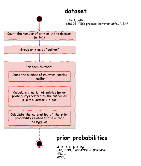
Learn the prior probability
The prior probability is learnt from the entries available in the training data using the following process …
calculate_prior_probabilities <- function(x){
  x %>%
    dplyr::group_by(author) %>%
    dplyr::count() %>%
    dplyr::ungroup() %>%
    dplyr::mutate(p_c = n/ sum(n)) %>%
    dplyr::mutate(p_c_log = log(p_c))
}


prior_probs_by_author <- calculate_prior_probabilities(spooky_training)
knitr::kable(prior_probs_by_author, format = "markdown")
| author | n | p_c | p_c_log |
|---|---|---|---|
| EAP | 5530 | 0.4034729 | -0.9076459 |
| HPL | 3945 | 0.2878301 | -1.2453847 |
| MWS | 4231 | 0.3086969 | -1.1753953 |
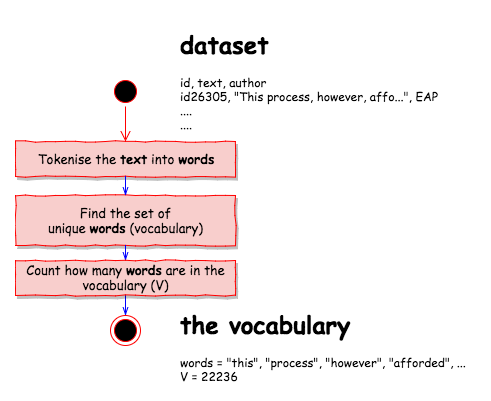
Learn the vocabulary $\mathbb{V}$
The vocabulary is learnt from the text made available in the training data using the following process …
get_vocabulary <- function(x){
  vocabulary <- x %>%
    tidytext::unnest_tokens(word, text) %>%
    dplyr::select(word) %>%
    dplyr::arrange(word)

  vocabulary <- unique(vocabulary$word)
  no_of_words <- length(vocabulary)

  return(list(words = vocabulary,
              V = no_of_words))
}

vocabulary <- get_vocabulary(spooky_training)
vocabulary_words <- vocabulary$words
V <- vocabulary$V
The vocabulary contains 22236 unique words like …
vocabulary_words[1:30]
##  [1] "a"            "à"            "a.d"          "a.m"
##  [5] "ab"           "aback"        "abaft"        "abandon"
##  [9] "abandoned"    "abandoning"   "abandonment"  "abaout"
## [13] "abasement"    "abashment"    "abate"        "abated"
## [17] "abatement"    "abating"      "abbé"         "abbey"
## [21] "abbreviation" "abdicated"    "abdication"   "abdications"
## [25] "abdomen"      "abdul"        "abernethy"    "aberrancy"
## [29] "aberrant"     "aberration"
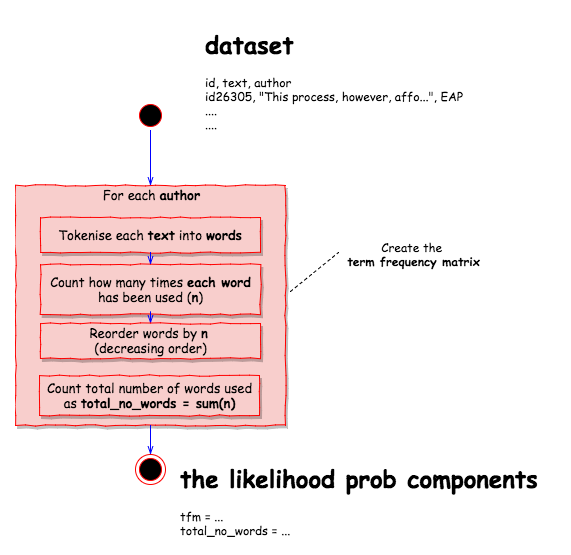
Learn the likelihood probability components
From the set of entries, made available for each author, is possible to calculate
- the frequency for each single word used by the author as ${count(w_i,author)}$ and,
- the total number of words used by the author as ${\sum_{w \in \mathbb{V}} count(w,author)}$
These components can then be used to calculate the likelihood probabilities $\hat P(w_i|author)$ for each word $w_i$ used by each author.
determine_terms_for <- function(x, y){
  tmp <- x %>%
    dplyr::filter(author == y) %>%
    dplyr::select(text) %>%
    tidytext::unnest_tokens(word, text) %>%
    dplyr::count(word) %>%
    dplyr::arrange(desc(n))

  return(list(tfm = tmp,
              total_no_words = sum(tmp$n)))
}

terms_EAP <- determine_terms_for(x = spooky_training, y = "EAP")
terms_HPL <- determine_terms_for(x = spooky_training, y = "HPL")
terms_MWS <- determine_terms_for(x = spooky_training, y = "MWS")
Edgard Allan Poe has used 140822 words and the term frequency matrix looks like
knitr::kable(terms_EAP$tfm[1:10,], format = "markdown")
| word | n |
|---|---|
| the | 10541 |
| of | 6285 |
| and | 4078 |
| to | 3326 |
| a | 3298 |
| in | 2883 |
| i | 2652 |
| it | 1600 |
| that | 1597 |
| was | 1514 |
HP Lovecraft has used 109814 words and the term frequency matrix looks like
knitr::kable(terms_HPL$tfm[1:10,], format = "markdown")
| word | n |
|---|---|
| the | 7625 |
| and | 4282 |
| of | 4063 |
| a | 2345 |
| to | 2284 |
| in | 1934 |
| i | 1857 |
| was | 1527 |
| that | 1419 |
| had | 1263 |
Mary Shelley has used 116898 words and the term frequency matrix looks like
knitr::kable(terms_MWS$tfm[1:10,], format = "markdown")
| word | n |
|---|---|
| the | 6798 |
| of | 4342 |
| and | 4330 |
| to | 3400 |
| i | 3024 |
| my | 1878 |
| a | 1846 |
| in | 1832 |
| was | 1571 |
| that | 1492 |
The implementation
train_nb_model <- function(dataset){
  learnt_prior_probs <- calculate_prior_probabilities(dataset)
  learnt_vocabulary <- get_vocabulary(dataset)

  learnt_terms_EAP <- determine_terms_for(x = dataset, y = "EAP")
  learnt_terms_HPL <- determine_terms_for(x = dataset, y = "HPL")
  learnt_terms_MWS <- determine_terms_for(x = dataset, y = "MWS")

  return(list(prior_probs = learnt_prior_probs,
              vocabulary = learnt_vocabulary,
              eap = learnt_terms_EAP,
              hpl = learnt_terms_HPL,
              mws = learnt_terms_MWS))
}
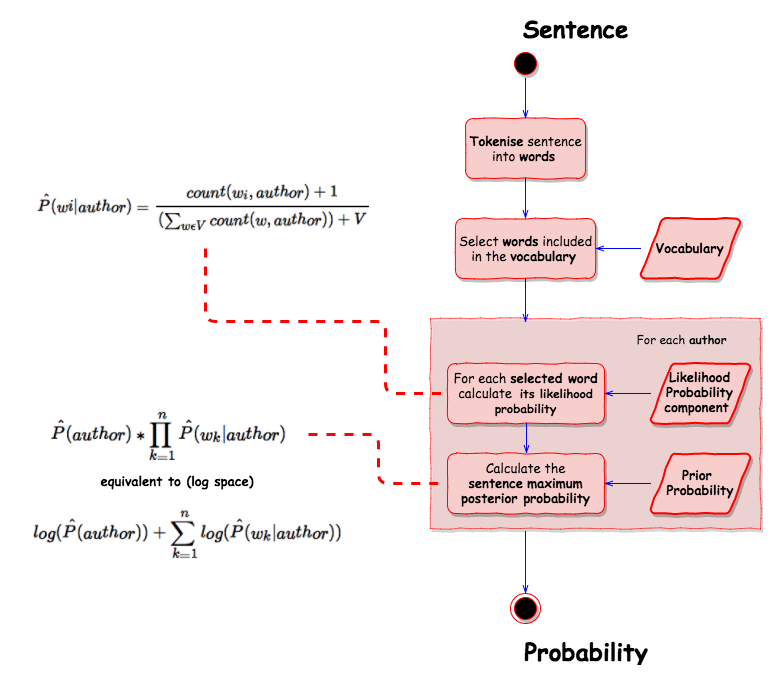
Calculate the probability of an author given a sentence/ excerpt
The prior probabilities, the vocabulary and the likelihood probability components can be used to estimate the maximum posterior probability $\hat P(author|sentence)$ for each author and for the provided sentence/ excerpt using the following process
Let’s take a sentence from the training dataset as example
“This process, however, afforded me no means of ascertaining the dimensions of my dungeon; as I might make its circuit, and return to the point whence I set out, without being aware of the fact; so perfectly uniform seemed the wall.”, by EAP
and walk through the process step by step.
First tokenise the sentence into relevant words (based on the vocabulary) …
tokenise_sentence_in_observation <- function(the_obs, the_vocabulary_terms){
  the_obs %>%
    tidytext::unnest_tokens(word, text) %>%
    dplyr::filter(word %in% the_vocabulary_terms) %>%
    dplyr::select(word)
}

sentence <- spooky_training[1,]

sentence_words <- tokenise_sentence_in_observation(
  the_obs = sentence,
  the_vocabulary_terms = vocabulary_words
)

sentence_words$word
##  [1] "this"         "process"      "however"      "afforded"
##  [5] "me"           "no"           "means"        "of"
##  [9] "ascertaining" "the"          "dimensions"   "of"
## [13] "my"           "dungeon"      "as"           "i"
## [17] "might"        "make"         "its"          "circuit"
## [21] "and"          "return"       "to"           "the"
## [25] "point"        "whence"       "i"            "set"
## [29] "out"          "without"      "being"        "aware"
## [33] "of"           "the"          "fact"         "so"
## [37] "perfectly"    "uniform"      "seemed"       "the"
## [41] "wall"
Once all the words have been identified, it is possible to calculate the likelihood probabilities for each word for a specific author (using Laplace smoothing for unknown words). For example for Edgard Allan Poe …
sentence_likelihood_probs_for_author <- function(the_sentence_words,
                                the_terms_for_author,
                                vocabulary_cardinality){
  no_terms <- sum(the_terms_for_author$n)

  the_sentence_words %>%
    dplyr::left_join(the_terms_for_author) %>%
    #set count to 0 if words is not used by the author
    dplyr::mutate(n = ifelse(is.na(n),0,n)) %>%
    #use Laplace smoothing
    dplyr::mutate(n_plus_1 = n + 1) %>%
    dplyr::mutate(p_w_c = n_plus_1 / (no_terms + vocabulary_cardinality)) %>%
    dplyr::mutate(p_w_c_log = log(p_w_c)) %>%
    dplyr::arrange(n)
}

likelihood_EAP <- sentence_likelihood_probs_for_author(sentence_words,
                           terms_EAP$tfm,
                           V)

knitr::kable(likelihood_EAP[1:8,], format = "markdown")
| word | n | n_plus_1 | p_w_c | p_w_c_log |
|---|---|---|---|---|
| uniform | 1 | 2 | 1.23e-05 | -11.308714 |
| ascertaining | 3 | 4 | 2.45e-05 | -10.615567 |
| circuit | 4 | 5 | 3.07e-05 | -10.392423 |
| process | 5 | 6 | 3.68e-05 | -10.210102 |
| whence | 5 | 6 | 3.68e-05 | -10.210102 |
| dungeon | 6 | 7 | 4.29e-05 | -10.055951 |
| dimensions | 7 | 8 | 4.91e-05 | -9.922420 |
| afforded | 12 | 13 | 7.97e-05 | -9.436912 |
… the word uniform has been used only 1 time (n) in the author corpus, its likelihood probability is 1.23e-05 (p_w_c), equivalent to -11.308714 (p_w_c_log) in the natural log space.
Finally the probability that the author is the writer given that sentence can be calculated using the priot probability and the likelihood probabilities …
calc_sentence_prob_log_for_author <- function(the_sentence_words,
                                          the_terms_for_author,
                                          vocabulary_cardinality,
                                          the_prior_prob){

  sentence_for <- sentence_likelihood_probs_for_author(the_sentence_words,
                                      the_terms_for_author,
                                      vocabulary_cardinality)
  return (the_prior_prob + sum(sentence_for$p_w_c_log))
}

# Calculate probability (log) for EAP
prob_log_EAP <- calc_sentence_prob_log_for_author(sentence_words,
    terms_EAP$tfm,
    V,
    prior_probs_by_author[prior_probs_by_author$author == "EAP",]$p_c_log)

print(paste("EAP prob:", prob_log_EAP, "(log),", exp(prob_log_EAP)))
## [1] "EAP prob: -272.839415045266 (log), 3.21623371427444e-119"
… and the probability that Edgard Allan Poe is the writer given that sentence is 3.2162337\times 10^{-119} (equivalent to -272.839415 in the natural log space).
The same can be done for the other authors HP Lovecraft and Mary Shelley (see below). The maximum posterior probability, for this specific sentence, is connected with Edgard Allan Poe, the actual writer of the sentence.
# Calculate probability (log) for HPL
prob_log_HPL <- calc_sentence_prob_log_for_author(sentence_words,
    terms_HPL$tfm,
    V,
    prior_probs_by_author[prior_probs_by_author$author == "HPL",]$p_c_log)

print(paste("HPL prob:", prob_log_HPL, "(log),", exp(prob_log_HPL)))
## [1] "HPL prob: -289.179819680819 (log), 2.5751351970092e-126"

# Calculate probability (log) for MWS
prob_log_MWS <- calc_sentence_prob_log_for_author(sentence_words,
    terms_MWS$tfm,
    V,
    prior_probs_by_author[prior_probs_by_author$author == "MWS",]$p_c_log)

print(paste("MWS prob:", prob_log_MWS, "(log),", exp(prob_log_MWS)))
## [1] "MWS prob: -288.379337717458 (log), 5.73383160825692e-126"
The implementation
calculate_probs_per_sentence <- function(entry, learnt_model){
  voc_words <- learnt_model$vocabulary$words
  voc_V <- learnt_model$vocabulary$V
  prior_probs <- learnt_model$prior_probs

  sentence_words <- entry %>%
    tidytext::unnest_tokens(word, text) %>%
    dplyr::filter(word %in% voc_words) %>%
    dplyr::select(word)

  eap_prob <- calc_sentence_prob_log_for_author(sentence_words,
                                            learnt_model$eap$tfm,
                                            voc_V,
                                            prior_probs[prior_probs$author == "EAP",]$p_c_log)

  hpl_prob <- calc_sentence_prob_log_for_author(sentence_words,
                                            learnt_model$hpl$tfm,
                                            voc_V,
                                            prior_probs[prior_probs$author == "HPL",]$p_c_log)

  mws_prob <- calc_sentence_prob_log_for_author(sentence_words,
                                            learnt_model$mws$tfm,
                                            voc_V,
                                            prior_probs[prior_probs$author == "MWS",]$p_c_log)

  pred_auth = "EAP"
  pred_max = eap_prob

  if(hpl_prob > pred_max){
    pred_auth = "HPL"
    pred_max = hpl_prob
  }

  if(mws_prob > pred_max){
    pred_auth = "MWS"
    pred_max = mws_prob
  }

  data.frame(id = entry$id,
             text = entry$text,
             auth = as.character(entry$author),
             EAP = eap_prob, HPL = hpl_prob, MWS = mws_prob,
             pred_auth = as.character(pred_auth),
             stringsAsFactors = F)

}
Some more examples ..
the_model <- train_nb_model(spooky_training)
res_1 <- calculate_probs_per_sentence(spooky_training[1,], the_model)
res_2 <- calculate_probs_per_sentence(spooky_training[10,], the_model)
res_3 <- calculate_probs_per_sentence(spooky_training[50,], the_model)
res_4 <- calculate_probs_per_sentence(spooky_training[100,], the_model)
res_5 <- calculate_probs_per_sentence(spooky_training[2,], the_model)
res <- rbind(res_1, res_2, res_3, res_4, res_5, stringsAsFactors = F)
knitr::kable(res, format = "markdown")
| id | text | auth | EAP | HPL | MWS | pred_auth |
|---|---|---|---|---|---|---|
| id26305 | This process, however, afforded me no means of ascertaining the dimensions of my dungeon; as I might make its circuit, and return to the point whence I set out, without being aware of the fact; so perfectly uniform seemed the wall. | EAP | -272.83941 | -289.17982 | -288.37934 | EAP |
| id18886 | The farm like grounds extended back very deeply up the hill, almost to Wheaton Street. | HPL | -119.12373 | -111.60003 | -122.83822 | HPL |
| id06377 | The stranger learned about twenty words at the first lesson; most of them, indeed, were those which I had before understood, but I profited by the others. | MWS | -177.04958 | -179.91193 | -176.38291 | MWS |
| id18834 | He reverted to his past life, his successes in Greece, his favour at home. | MWS | -106.25498 | -102.13303 | -96.80837 | MWS |
| id17569 | It never once occurred to me that the fumbling might be a mere mistake. | HPL | -91.45167 | -93.29227 | -94.69620 | EAP |
Evaluating the model
The evaluation of the model is done using the spooky_testing dataset, that has not been used for the training of the model. Some info about the testing dataset …
# Total no of entries
dim(spooky_testing)[1]
## [1] 5873

# No of entries by authors
table(spooky_testing$author)
##
##  EAP  HPL  MWS
## 2370 1690 1813

# % of entries by authors
round(100 * prop.table(table(spooky_testing$author)), digits = 2)
##
##   EAP   HPL   MWS
## 40.35 28.78 30.87
Using the training model, the author prediction is done for each entry in the testing data …
res <- NULL
for (i in seq_along(spooky_testing$id)){
  tmp <- calculate_probs_per_sentence(spooky_testing[i,], the_model)
  if(is.null(res)){
    res <- tmp
  }else{
    res <- rbind(res, tmp)
  }
}

res$EAP <- exp(res$EAP)
res$HPL <- exp(res$HPL)
res$MWS <- exp(res$MWS)
The confusion matrix (with some relevant metrics) and the F1-score are used to estimate how good the model is.
#pred. vs. truth
caret::confusionMatrix(res$pred_auth, res$auth)
## Confusion Matrix and Statistics
##
##           Reference
## Prediction  EAP  HPL  MWS
##        EAP 1950  208  171
##        HPL  138 1370   81
##        MWS  282  112 1561
##
## Overall Statistics
##
##                Accuracy : 0.8311
##                  95% CI : (0.8213, 0.8406)
##     No Information Rate : 0.4035
##     P-Value [Acc > NIR] : < 2.2e-16
##
##                   Kappa : 0.7438
##  Mcnemar's Test P-Value : 4.802e-10
##
## Statistics by Class:
##
##                      Class: EAP Class: HPL Class: MWS
## Sensitivity              0.8228     0.8107     0.8610
## Specificity              0.8918     0.9476     0.9030
## Pos Pred Value           0.8373     0.8622     0.7985
## Neg Pred Value           0.8815     0.9253     0.9357
## Prevalence               0.4035     0.2878     0.3087
## Detection Rate           0.3320     0.2333     0.2658
## Detection Prevalence     0.3966     0.2706     0.3329
## Balanced Accuracy        0.8573     0.8791     0.8820
table_pred_vs_truth <- table(res$pred_auth, res$auth)
caret::F_meas(table_pred_vs_truth)
## [1] 0.8299638
References
[1] Kaggle challenge: Spooky AUthor Identification
To have a better overview and understanding of the theory behind text classification & Naive Bayes classifiers, the material created by Dan Jurafsky & Christopher Manning for the “Natural Language Processing” MOOC at Coursera is a great starting point
-
Lesson Videos
The “Speech and Language Processing” book of Dan Jurafsky & James H. Martin
- “Naive Bayes and Sentiment Classification” chapter
Session Info
## R version 3.3.3 (2017-03-06)
## Platform: x86_64-apple-darwin13.4.0 (64-bit)
## Running under: macOS  10.13.1
##
## locale:
## [1] no_NO.UTF-8/no_NO.UTF-8/no_NO.UTF-8/C/no_NO.UTF-8/no_NO.UTF-8
##
## attached base packages:
## [1] stats     graphics  grDevices utils     datasets  methods   base
##
## other attached packages:
## [1] bindrcpp_0.2    caret_6.0-77    ggplot2_2.2.1   lattice_0.20-35
## [5] tidytext_0.1.5  dplyr_0.7.4     readr_1.1.1
##
## loaded via a namespace (and not attached):
##  [1] Rcpp_0.12.13       lubridate_1.7.1    tidyr_0.7.2
##  [4] class_7.3-14       assertthat_0.2.0   rprojroot_1.2
##  [7] digest_0.6.12      ipred_0.9-6        psych_1.7.8
## [10] foreach_1.4.3      R6_2.2.2           plyr_1.8.4
## [13] backports_1.1.1    stats4_3.3.3       e1071_1.6-8
## [16] evaluate_0.10.1    highr_0.6          rlang_0.1.4
## [19] lazyeval_0.2.1     kernlab_0.9-25     rpart_4.1-11
## [22] Matrix_1.2-12      rmarkdown_1.8      splines_3.3.3
## [25] CVST_0.2-1         ddalpha_1.3.1      gower_0.1.2
## [28] stringr_1.2.0      foreign_0.8-69     munsell_0.4.3
## [31] broom_0.4.2        janeaustenr_0.1.5  pkgconfig_2.0.1
## [34] mnormt_1.5-5       dimRed_0.1.0       htmltools_0.3.6
## [37] nnet_7.3-12        tibble_1.3.4       prodlim_1.6.1
## [40] DRR_0.0.2          codetools_0.2-15   RcppRoll_0.2.2
## [43] withr_2.1.0        MASS_7.3-47        recipes_0.1.0
## [46] ModelMetrics_1.1.0 SnowballC_0.5.1    grid_3.3.3
## [49] nlme_3.1-131       gtable_0.2.0       magrittr_1.5
## [52] scales_0.5.0       tokenizers_0.1.4   stringi_1.1.6
## [55] reshape2_1.4.2     timeDate_3042.101  robustbase_0.92-8
## [58] lava_1.5.1         iterators_1.0.8    tools_3.3.3
## [61] glue_1.2.0         DEoptimR_1.0-8     purrr_0.2.4
## [64] sfsmisc_1.1-1      hms_0.3            parallel_3.3.3
## [67] survival_2.41-3    yaml_2.1.14        colorspace_1.3-2
## [70] knitr_1.17         bindr_0.1