The content of this blog is based on examples/ notes/ experiments related to the material presented in the “Building Data Visualization Tools” module of the “Mastering Software Development in R” Specialization (Coursera) created by Johns Hopkins University [1].
Required Packages
ggplot2, a system for ‘declaratively’ creating graphics, based on “The Grammar of Graphics”.gridExtra, provides a number of user-level functions to work with “grid” graphics.dplyr, a tool for working with data frame like objects, both in memory and out of memory.viridis, the viridis color palette.ggmap, a collection of functions to visualize spatial data and models on top of static maps from various online sources (e.g Google Maps)
# If necessary to install a package run
# install.packages("packageName")

# Load packages
library(ggplot2)
library(gridExtra)
library(dplyr)
library(viridis)
library(ggmap)
Data
The ggplot2 package includes some datasets with geographic information. The ggplot2::map_data() function allows to get map data from the maps package (use ?map_data form more information).
Specifically the italy dataset [2] is used for some of the examples below. Please note that this dataset was prepared aroind 1989 so it is out of date especially information pertaining provinces (see ?maps::italy).
# Get the italy dataset from ggplot2
# Consider only the following provinces "Bergamo" , "Como", "Lecco", "Milano", "Varese"
# and arrange by group and order (ascending order)
italy_map <- ggplot2::map_data(map = "italy")
italy_map_subset <- italy_map %>%
  filter(region %in% c("Bergamo" , "Como", "Lecco", "Milano", "Varese")) %>%
  arrange(group, order)
Each observation in the dataframe defines a geographical point with some extra information:
long&lat, longitude and latitude of the geographical pointgroup, an identifier connected with the specific polygon points are part of- a map can be made of different polygons (e.g. one polygon for the main land and one for each islands, one polygon for each state, …)
order, the order of the point within the specificgroup- how the all of the points being part of the same
groupshould be connected in order to create the polygon
- how the all of the points being part of the same
region, the name of the province (Italy) or state (USA)
head(italy_map, 3)
##       long      lat group order        region subregion
## 1 11.83295 46.50011     1     1 Bolzano-Bozen      <NA>
## 2 11.81089 46.52784     1     2 Bolzano-Bozen      <NA>
## 3 11.73068 46.51890     1     3 Bolzano-Bozen      <NA>
How to work with maps
Having spatial information in the data gives the opportunity to map the data or, in other words, visualizing the information contained in the data in a geographical context. R has different possibilities to map data, from normal plots using longitude/ latitude as x/ y to more complex spatial data objects (e.g. shapefiles).
Mapping with ggplot2 package
The most basic way to create maps with your data is to use ggplot2, create a ggplot object and then, add a specific geom mapping longitute to x aesthetic and latitude to y aesthetic [4] [5]. This simple approach can be used to:
- create maps of geographical areas (states, country, etc.)
- map locations as points, lines, etc.
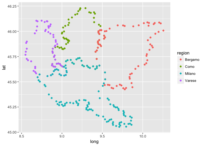
Create a map showing “Bergamo”, Como”, “Varese” and “Milano” provinces in Italy using simple points…
When plotting simple points the geom_point function is used. In this case the polygon and order of the points is not important when plotting.
italy_map_subset %>%
  ggplot(aes(x = long, y = lat)) +
  geom_point(aes(color = region))
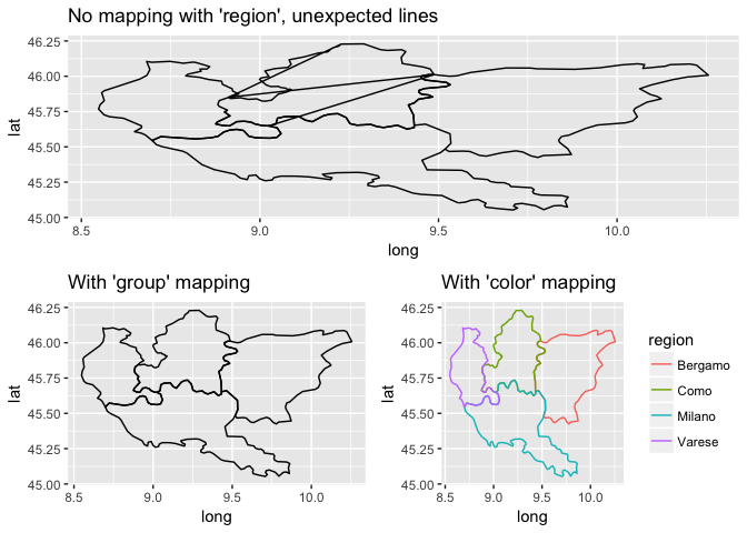
Create a map showing “Bergamo”, Como”, “Varese” and “Milano” provinces in Italy using lines…
The geom_path function is used to create such plots. From the R documentation, geom_path “… connects the observation in the order in which they appear in the data”. When plotting using geom_path is important to consider the polygon and the order within the polygon for each point in the map.
The points in the dataset are grouped by region and ordered by order. If information about the region is not provided then the sequential order of the observations will be the order used to connect the points and, for this reason, “unexpected” lines will be drawn when moving from a region to the other. On the other hand if information about the region is provided using the group or color aesthetic, mapping to region, the “unexpected” lines are removed (see example below).
plot_1 <- italy_map_subset %>%
  ggplot(aes(x = long, y = lat)) +
  geom_path() +
  ggtitle("No mapping with 'region', unexpected lines")

plot_2 <- italy_map_subset %>%
  ggplot(aes(x = long, y = lat)) +
  geom_path(aes(group = region)) +
  ggtitle("With 'group' mapping")

plot_3 <- italy_map_subset %>%
  ggplot(aes(x = long, y = lat)) +
  geom_path(aes(color = region)) +
  ggtitle("With 'color' mapping")

grid.arrange(plot_1, plot_2, plot_3, ncol = 2, layout_matrix = rbind(c(1,1), c(2,3)))
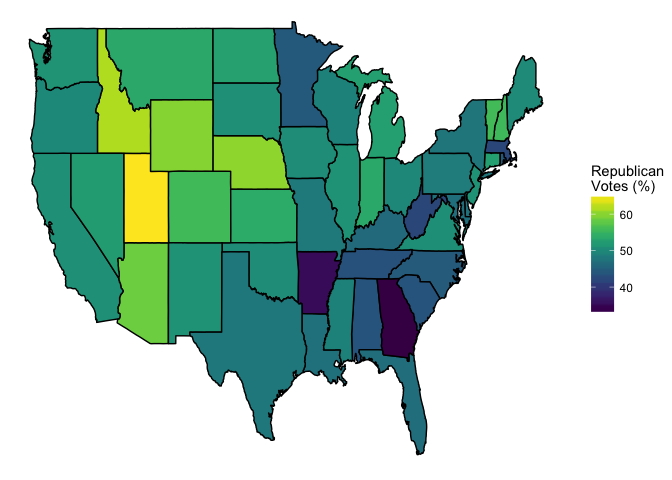
Mapping with ggplot2 is possible to create more sophisticated maps like choropleth maps [3]. The example below, extracted from [1], shows how to visualize the percentage of republican votes in 1976 by states.
# Get the USA/ state map from ggplot2
us_map <- ggplot2::map_data("state")

# Use the 'votes.repub' dataset (maps package), containing the percentage of
# republican votes in the 1900 elections by state. Note
# - the dataset is a matrix so it needs to be converted to a dataframe
# - the row name defines the relevant state

votes.repub %>%
  tbl_df() %>%
  mutate(state = rownames(votes.repub), state = tolower(state)) %>%
  right_join(us_map, by = c("state" = "region")) %>%
  ggplot(mapping = aes(x = long, y = lat, group = group, fill = `1976`)) +
  geom_polygon(color = "black") +
  theme_void() +
  scale_fill_viridis(name = "Republican\nVotes (%)")
Maps with ggmap package, Google Maps API and others
Another way to create maps is to use the ggmap[4] package (see Google Maps API Terms of Service). As stated in the package description
“A collection of functions to visualize spatial data and models on top of static maps from various online sources (e.g Google Maps,..). It includes tools common to those tasks, including functions for geolocation and routing.” R Documentation
The package allows to create/ plot maps using Google Maps and few other service providers, and perform some other interesting tasks like geocoding, routing, distance calculation, etc. The maps are actually ggplot objects making possible to reuse the ggplot2 functionality like adding layers, modify the theme, …
“The basic idea driving ggmap is to take a downloaded map image, plot it as a context layer using ggplot2, and then plot additional content layers of data, statistics, or models on top of the map. In ggmap this process is broken into two pieces – (1) downloading the images and formatting them for plotting, done with get_map, and (2) making the plot, done with ggmap. qmap marries these two functions for quick map plotting (c.f. ggplot2’s ggplot), and qmplot attempts to wrap up the entire plotting process into one simple command (c.f. ggplot2’s qplot).” [4]
How to create and plot a map…
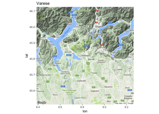
The ggmap::get_mapfunction is used to get a base map (a ggmap object, a raster object) from different service providers like Google Maps, OpenStreetMap, Stamen Maps or Naver Maps (default setting is Google Maps). Once the base map is available, then it can been plotted using the ggmap::ggmap function. Alternatively the ggmap::qmap function (quick map plot) can be used.
# When querying for a base map the location must be provided
# name, address (geocoding)
# longitude/ latitude pair
base_map <- get_map(location = "Varese")
ggmap(base_map) + ggtitle("Varese")
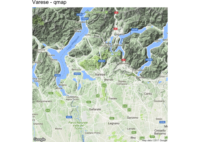
# qmap is a wrapper for
# `ggmap::get_map` and `ggmap::ggmap` functions.
qmap("Varese") + ggtitle("Varese - qmap")
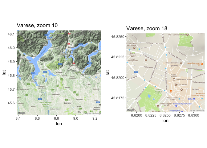
How to change the zoom in the map…
The zoom argument (default value is auto) in ggmap::get_map function can be used to control the zoom of the returned base map (see ?get_map for more information). Please note that the possible values/ range for the zoom argument changes with the different sources.
# An example using Google Maps as a source
# Zoom is an integer between 3 - 21 where
# zoom = 3 (continent)
# zoom = 10 (city)
# zoom = 21 (building)

base_map_10 <- get_map(location = "Varese", zoom = 10)
base_map_18 <- get_map(location = "Varese", zoom = 16)

grid.arrange(ggmap(base_map_10) + ggtitle("Varese, zoom 10"),
             ggmap(base_map_18) + ggtitle("Varese, zoom 18"),
             nrow = 1)
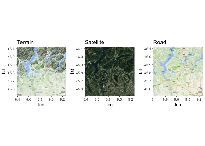
How to change the type of map…
The maptype argument in ggmap::get_map function can be used to change the type of map aka map theme. Based on the R documentation (see ?get_map for more information)
‘[maptype]… options available are “terrain”, “terrain-background”, “satellite”, “roadmap”, and “hybrid” (google maps), “terrain”, “watercolor”, and “toner” (stamen maps)…’.
# An example using Google Maps as a source
# and different map types

base_map_ter <- get_map(location = "Varese", maptype = "terrain")
base_map_sat <- get_map(location = "Varese", maptype = "satellite")
base_map_roa <- get_map(location = "Varese", maptype = "roadmap")

grid.arrange(ggmap(base_map_ter) + ggtitle("Terrain"),
             ggmap(base_map_sat) + ggtitle("Satellite"),
             ggmap(base_map_roa) + ggtitle("Road"),
             nrow = 1)
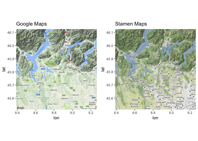
How to change the source for maps…
While the default source for maps with ggmap::get_map is Google Maps, it is possible to change the map service using the source argument. The supported map services/ sources are Google Maps, OpenStreeMaps, Stamen Maps and CloudMade Maps (see ?get_map for more information).
# An example using different map services as a source

base_map_google <- get_map(location = "Varese", source = "google", maptype = "terrain")
base_map_stamen <- get_map(location = "Varese", source = "stamen", maptype = "terrain")

grid.arrange(ggmap(base_map_google) + ggtitle("Google Maps"),
             ggmap(base_map_stamen) + ggtitle("Stamen Maps"),
             nrow = 1)
How to geocode a location…
The ggmap::geocode function can be used to find latitude and longitude of a location based on its name (see ?geocode for more information). Note that Google Maps API limits the possible number of queries per day, geocodeQueryCheck can be used to determine how many queries are left.
# Geocode a city
geocode("Sesto Calende")
##        lon     lat
## 1 8.636597 45.7307
# Geocode a set of cities
geocode(c("Varese", "Milano"))
##        lon     lat
## 1 8.825058 45.8206
## 2 9.189982 45.4642

# Geocode a location
geocode(c("Milano", "Duomo di Milano"))
##        lon     lat
## 1 9.189982 45.4642
## 2 9.191926 45.4641
geocode(c("Roma", "Colosseo"))
##        lon      lat
## 1 12.49637 41.90278
## 2 12.49223 41.89021
How to find a route between two locations…
The ggmap::route function can be used to find a route from Google using different possible modes, e.g. walking, driving, … (see ?ggmap::route for more information).
‘The route function provides the map distances for the sequence of “legs” which constitute a route between two locations. Each leg has a beginning and ending longitude/latitude coordinate along with a distance and duration in the same units as reported by mapdist. The collection of legs in sequence constitutes a single route (path) most easily plotted with geom_leg, a new exported ggplot2 geom…’ [4]
route_df <- route(from = "Somma Lombardo", to = "Sesto Calende", mode = "driving")
head(route_df)
##      m    km     miles seconds   minutes       hours startLon startLat
## 1  198 0.198 0.1230372      52 0.8666667 0.014444444 8.706770 45.68277
## 2  915 0.915 0.5685810     116 1.9333333 0.032222222 8.705170 45.68141
## 3  900 0.900 0.5592600      84 1.4000000 0.023333333 8.702070 45.68835
## 4 5494 5.494 3.4139716     390 6.5000000 0.108333333 8.691054 45.69019
## 5  205 0.205 0.1273870      35 0.5833333 0.009722222 8.648636 45.72250
## 6  207 0.207 0.1286298      25 0.4166667 0.006944444 8.649884 45.72396
##     endLon   endLat leg
## 1 8.705170 45.68141   1
## 2 8.702070 45.68835   2
## 3 8.691054 45.69019   3
## 4 8.648636 45.72250   4
## 5 8.649884 45.72396   5
## 6 8.652509 45.72367   6
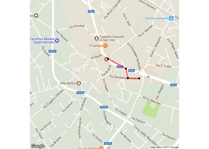
route_df <- route(from = "Via Gerolamo Fontana 32, Somma Lombardo",
                  to = "Town Hall, Somma Lombardo", mode = "walking")

qmap("Somma Lombardo", zoom = 16) +
  geom_leg(
    aes(x = startLon, xend = endLon, y = startLat, yend = endLat),  colour = "red",
    size = 1.5, alpha = .5,
    data = route_df) +
  geom_point(aes(x = startLon, y = startLat), data = route_df) +
  geom_point(aes(x = endLon, y = endLat), data = route_df)
How to find the distance between two locations…
The ggmap::mapdist function can be used to compute the distance between two location using different possible modes, e.g. walking, driving, … (see ?ggmap::mapdist for more information).
# Driving
mapdist(from = "Somma Lombardo", to = "Sesto Calende", mode = "driving")
##             from            to    m    km    miles seconds  minutes
## 1 Somma Lombardo Sesto Calende 9947 9.947 6.181066     988 16.46667
##       hours
## 1 0.2744444
# Walking
mapdist(from = "Somma Lombardo", to = "Sesto Calende", mode = "walking")
##             from            to    m    km    miles seconds minutes  hours
## 1 Somma Lombardo Sesto Calende 8734 8.734 5.427308    6597  109.95 1.8325
More on mapping
- Using the
choroplethrandchoroplethrMapspackages, see “Mapping US counties and states” section in [1] - Working with spatial objects and shapefiles, see “More advanced mapping – Spatial objects” section in [1]
- Using htmlWidgets for mapping in R using leaflet [5]
References
[1] “Mapping” chapter in “Mastering Software Development in R” by Roger D. Peng, Sean Cross and Brooke Anderson, 2017
[2] Italy Map, “UNESCO (1987) through UNEP/GRID-Geneva”
[3] Choropleth map Wikipedia
[4] D. Kahle and H. Wickham. ggmap: Spatial Visualization with ggplot2. The R Journal, 5(1), 144-161.
[5] Using Leaflet for R
Previous “Building Data Visualization Tools” blogs
[6] “Basic plotting with R and ggplot2”, Part 1
[7] “‘ggplot2’, essential concepts”, Part 2
[8] “Guidelines for good plots”, Part 3