The content of this blog is based on examples/ notes/ experiments related to the material presented in the “Building Data Visualization Tools” module of the “Mastering Software Development in R” Specialization (Coursera) created by Johns Hopkins University [1].
Required packages:
- the
gridpackage, - the
ggplot2package, - …
# Note that the grid package is a base package
# it is installed automatically when installing R
library(grid)

# If ggplot2 package is not installed
# install.packages("ggplot2")
library(ggplot2)
1. The grid package and the grid graphic system
The core package, supporting the graphics capabilities in R, is the grDevices package. Two packages are built directly on this engine, the graphics and the grid packages - two different and incompatible graphic systems (see picture below for more information).
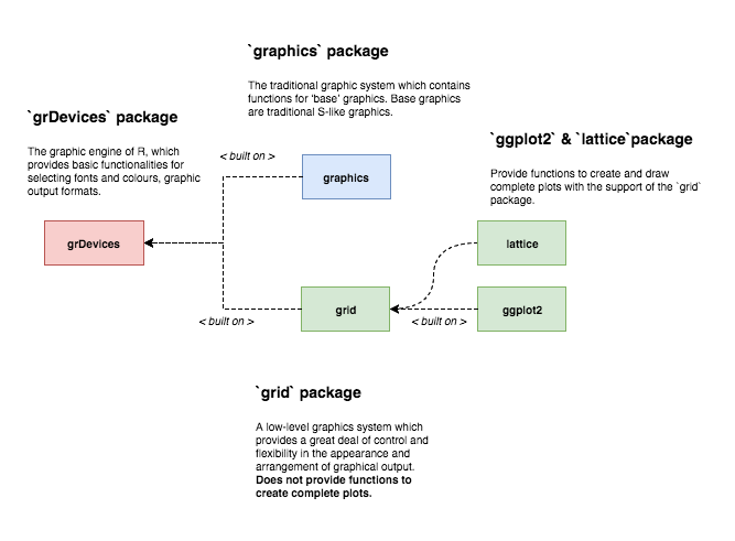
The ggplot2 package is built on top of the grid graphic system. The grid package provides the primitive functions that are used by ggplot2 for creating and drawing complete plots. While it is not required to interact directly with the grid package, it is necessary to understand how it does work in order to be able to create and add customizations not supported by ggplot2.
As stated in [2]
“grid is a low-level graphics system which provides a great deal of control and flexibility in the appearance and arrangement of graphical output. grid does not provide high-level functions which create complete plots. What it does provide is a basis for developing such high-level functions (e.g., the lattice and ggplot2 packages), the facilities for customising and manipulating lattice output, the ability to produce high-level plots or non-statistical images from scratch, and the ability to add sophisticated annotations to the output from base graphics functions (see the gridBase package).”
The grid graphic system provides only low-level graphic functions that can be used to create basic graphical features and it does not provide high level functions for producing complete plots. Please note that there are two different families of functions in the grid package
*Grob()family of functions, used to create grobs as R objects, andgrid.*()family of functions, used to create grobs as graphical output.
The main focus in this blog is to use grobs as R objects. The list of the *Grob() family of functions used for such purpouse can be found below
ls(name = "package:grid", pattern = ".*Grob")
##  [1] "addGrob"       "arrowsGrob"    "bezierGrob"    "circleGrob"
##  [5] "clipGrob"      "curveGrob"     "editGrob"      "forceGrob"
##  [9] "frameGrob"     "functionGrob"  "getGrob"       "legendGrob"
## [13] "linesGrob"     "lineToGrob"    "moveToGrob"    "nullGrob"
## [17] "packGrob"      "pathGrob"      "placeGrob"     "pointsGrob"
## [21] "polygonGrob"   "polylineGrob"  "rasterGrob"    "rectGrob"
## [25] "removeGrob"    "reorderGrob"   "roundrectGrob" "segmentsGrob"
## [29] "setGrob"       "showGrob"      "textGrob"      "xaxisGrob"
## [33] "xsplineGrob"   "yaxisGrob"
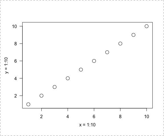
It is possible to combine these low-level functions to create complete plots (even if not not recommended). See the following example (adapted from [2])
# scatterplot example
# create scatterplot plot(1:10)
# using the grid package

# create and draw a rectangle - line type = dashed
gRect1 <- rectGrob(gp = gpar(lty = "dashed"))
grid.draw(gRect1)
# create the data points
x <- y <- 1:10
# create a viewport providing the margins as number of text lines
vp1 <- plotViewport(c(5.1,4.1,4.1,2.1))
# navigate into the created viewport
pushViewport(vp1)
# create a viewport with x and y scales
# based on provided values
dvp1 <- dataViewport(x,y)
# navigate into the created viewport
pushViewport(dvp1)
# create and draw a rectangle
gRect2 <- rectGrob()
grid.draw(gRect2)
# create and draws the x and y axis
gXaxis <- xaxisGrob()
grid.draw(gXaxis)
gYaxis <- yaxisGrob()
grid.draw(gYaxis)
# create and draw the data points
gPoints <- pointsGrob(x,y)
grid.draw(gPoints)
# create and draw text
gYText <- textGrob("y = 1:10", x = unit(-3, "lines"), rot = 90)
grid.draw(gYText)
gXText <- textGrob("x = 1:10", y = unit(-3, "lines"))
grid.draw(gXText)
# exit the 2 viewports
popViewport(2)
2. The grid graphic system: basic concepts
2.1 Grobs: graphical objects
The most critical concept to understand is the grob. A grob is a grid graphical object that can be created, changed and plotted using the grid graphic functions. Grobs are
- created,
- modified,
- added or removed from larger grid objects (optionally) and
- drawn on a graphics device.
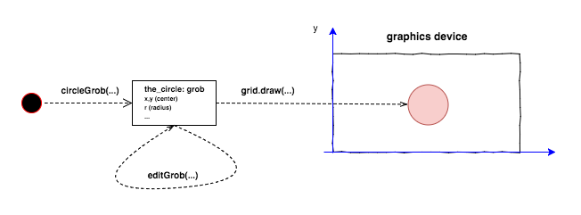
Possible grobs include circles, lines, points, rectangles, polygons, etc. Once a grob is created, it can be modified (using the editGrob function) and then drawn (using the grid.draw function) on a graphics device.
When creating a grob the location where the grob should be places/ located must be provided. As an examples the circleGrob accepts the following arguments (see ?circleGrob for more details):
x, a numeric vectors specifying the x location (center of the circle)y, a numeric vectors specifying the y location (center of the circle)r, , a numeric vectors specifying the radius of the circledefault.units, a string indicating the default units to use.
See examples below for some examples.
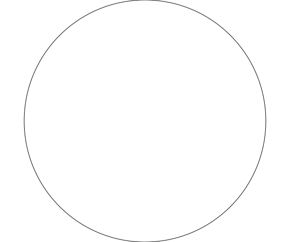
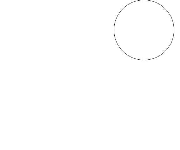
# Create a circle grob object and draw it in the current device
# See ?circleGrob for possible arguments and default values
grid.newpage() # Erase/ clear the current device
the_circle <- circleGrob() # Create the circe grob
grid.draw(the_circle) # Draw the grob (current device)
# Create a circle grob object with specific settings (center and radius)
# modify the object (center and radius) and draw it
grid.newpage()
the_circle <- circleGrob(x = 0.2, y = 0.2, r = 0.2)
the_circle <- editGrob(the_circle,
                       x = unit(0.8, "npc"),
                       y = unit(0.8, "npc"),
                       r = unit(0.2, "npc"))
grid.draw(the_circle)
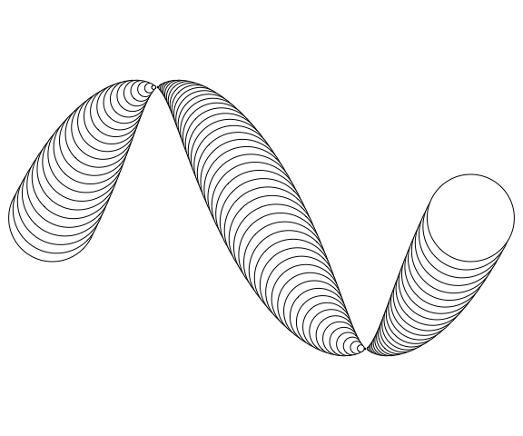
# Create a circle grob object
# using the power of vectorization
grid.newpage() # Erase/ clear the current device
the_circle <- circleGrob(
  x = seq(0.1, 0.9, length = 100),
  y = 0.5 + 0.3 * sin(seq(0, 2*pi, length = 100)),
  r = abs(0.1 * cos(seq(0, 2*pi, length = 100)))
)
grid.draw(the_circle)
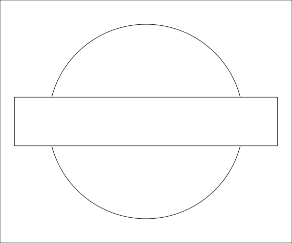
More grob objects can be plot on the same device as part of the same visualization/ graph, your fantasy becomes your limit …
grid.newpage() # Erase/ clear the current device

outer_rectangle <- rectGrob()
my_circle <- circleGrob(x = 0.5, y = 0.5, r = 0.4)
my_rect <- rectGrob(width = 0.9, height = 0.2)

grid.draw(outer_rectangle)
grid.draw(my_circle)
grid.draw(my_rect)
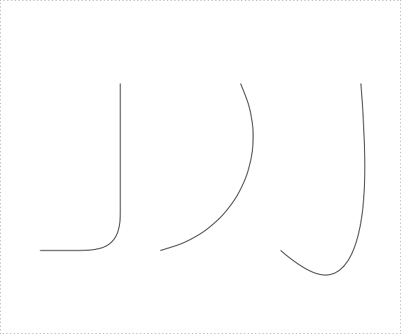
grid.newpage() # Erase/ clear the current device
outer_rectangle <- rectGrob(gp = gpar(lty = 3))
curve_1 <- curveGrob(x1 = 0.1, y1 = 0.25, x2 = 0.3, y2 = 0.75)
curve_2 <- curveGrob(x1 = 0.4, y1 = 0.25, x2 = 0.6, y2 = 0.75, square = F, ncp = 8, curvature = 0.5)
curve_3 <- curveGrob(x1 = 0.7, y1 = 0.25, x2 = 0.9, y2 = 0.75, square = F, angle = 45, shape = -1)

grid.draw(outer_rectangle)
grid.draw(curve_1)
grid.draw(curve_2)
grid.draw(curve_3)
2.1.1 Controlling the appearance of a grob: the argument: gp
All these functions, used to create grobs, accept a gp argument that is used to control some aspects of the graphical parameter like
- colour of lines and borders,
- colour for fillings of rectangles and polygons,
- line type,
- trasparency,
- etc.
To see the list of the possible aspects that can be controlled using the gp argument see the ?gpar help page.
grid.newpage() # Erase/ clear the current device

outer_rectangle <- rectGrob()
my_circle <- circleGrob(x = 0.5, y = 0.5, r = 0.4,
                        gp = gpar(col = "black", lty = 1, fill = "blue"))
my_rect <- rectGrob(width = 0.9, height = 0.2,
                    gp = gpar(col = "black", lty = 1, fill = "red"))

grid.draw(outer_rectangle)
grid.draw(my_circle)
grid.draw(my_rect)
2.1.2 The gTree object
A gTree object is a grob that can have other grobs as children. It is useful to create grobs that are made of multiple elements (e.g. like a scatterplot). When a gTree object is drawn, all of its children are drawn. See the example below…
grid.newpage() # Erase/ clear the current device
circle_1_1 <- circleGrob(name = "circle_1_1",
                         x = 0.1, y = 0.8, r = 0.1)
circle_1_2 <- circleGrob(name = "circle_1_2",
                         x = 0.1, y = 0.8, r = 0.05,
                         gp = gpar(fill = "red"))
circle_1 <- gTree(name = "circle_1_tree", children = gList(circle_1_1, circle_1_2))


circle_2_1 <- circleGrob(x = 0.9, y = 0.8, r = 0.1)
circle_2_2 <- circleGrob(x = 0.9, y = 0.8, r = 0.05,
                         gp = gpar(fill = "red"))
circle_2 <- gTree(children = gList(circle_2_1, circle_2_2))

circle_3_1 <- circleGrob(x = 0.5, y = 0.2, r = 0.1)
circle_3_2 <- circleGrob(x = 0.5, y = 0.2, r = 0.05,
                         gp = gpar(fill = "red"))
circle_3 <- gTree(children = gList(circle_3_1, circle_3_2))

line_1 <- linesGrob(x = c(0.1, 0.5),
                    y = c(0.8,0.6),
                    gp = gpar(lwd = 4))
line_2 <- linesGrob(x = c(0.9, 0.5),
                    y = c(0.8,0.6),
                    gp = gpar(lwd = 4))
line_3 <- linesGrob(x = c(0.5, 0.5),
                    y = c(0.6,0.2),
                    gp = gpar(lwd = 4))
the_text <- textGrob("Flux Capacitator",
                     x = 0.5, y = 0.9)

flux_capacitator <- gTree(
  children = gList(circle_1, circle_2, circle_3,
                   line_1, line_2, line_3, the_text)
  )
grid.draw(flux_capacitator)
The function grid.ls() can be used to have a listing of the grobs that are part of the structure in the current graphic device. Note how the grobs name is used in the returned listing, if a name parameter was provided when creating a grob such name is used to identify the grob in the listing (e.g. the circle_1 gTree and its children).
grid.ls(flux_capacitator)
## GRID.gTree.31
##   circle_1_tree
##     circle_1_1
##     circle_1_2
##   GRID.gTree.23
##     GRID.circle.21
##     GRID.circle.22
##   GRID.gTree.26
##     GRID.circle.24
##     GRID.circle.25
##   GRID.lines.27
##   GRID.lines.28
##   GRID.lines.29
##   GRID.text.30
2.2 Viewports
A viewport is a rectangular region that provides a context for drawing, specifically,
- a geometric context consisting in a coordinate system for location and
- a graphical context consisting of explicit graphical parameter settings to control the appearance of the output.
As stated in the vignettes [2,3], a viewport is defined as a graphics region that you can move into and out of to customize plots. Viewports can be created inside another viewport and so on.
By default grid creates a root viewport that correspond to the entire device, so the actual drawing is within the full device till another viewport is added (creating a viewport tree). There is always one and only one current viewport at any time.
2.2.1 How to create a viewport
A viewport can be created using the Viewport function. A viewport has a location (x, y arguments), a size (width, height arguments) and a justification (just argument) - see ?Viewport for more information. No region is created on the device till the viewport is navigated into.
grid.newpage() # Erase/ clear the current device
viewport_1 <- viewport(x = 0.5, y = 0.5,
                       width = 0.5, height = 0.5,
                       just = c("left", "bottom"))

# viewport_1 is a "viewport" object
# No region has been actually created on the device
viewport_1
## viewport[GRID.VP.3]
class(viewport_1)
## [1] "viewport"
2.2.2 How to work with viewports
Using the grid graphic system, plots can be created using viewports (viewports and nested viewports), specifically creating new viewports, navigating into them and drawing grobs and then moving to a different viewport, so on and on.
The pushViewport() and popViewport() functions can be used, respectively, to navigate into a viewport (changing the current viewport), and to navigate out of the current viewport. When a viewport is popped, the drawing context reverts to the parent viewport and the viewport is removed from the device.
grid.newpage() # Erase/ clear the current device
# By default a root viewport is created
# and set as the current one

# Create a new viewport
viewport_1 <- viewport(name = "vp1",
                       width = 0.5, height = 0.3,
                       angle = 10)

# Working on the root viewport
grid.draw(rectGrob(name = "root_rect"))
grid.draw(textGrob(name = "root_text",
          "Board", x = unit(1, "mm"),
          y = unit(1, "npc") - unit(1, "mm"),
          just = c("left", "top")))

# Move into the created viewport
# Current viewport is switch to vp1
pushViewport(viewport_1)
# Draw into the current viewport
grid.draw(rectGrob(name = "vp1_rect"))
grid.draw(textGrob(name = "vp1_text",
          "Task 1", x = unit(1, "mm"),
          y = unit(1, "npc") - unit(1, "mm"),
          just = c("left", "top")))

pushViewport(viewport_1)
# Draw into the current viewport
grid.draw(rectGrob(name = "vp1_vp1_rect"))
grid.draw(textGrob(name = "vp1_vp1_text",
          "Task 1", x = unit(1, "mm"),
          y = unit(1, "npc") - unit(1, "mm"),
          just = c("left", "top")))
# Move out of the current viewport
# back to the root (set as current)
popViewport()

# Move out of the current viewport
# back to the root (set as current)
popViewport()
Another way to change the current viewport is by using the upViewport() and downViewport() functions. The upViewport() function is similar to popViewport()with the difference that upViewport() does not remove the current viewport from the device (more efficient and fast).
2.3 Coordinate systems
When creating a grid graphical object or a viewport object, the location of where this object should be located and its size must be provided (e.g. through x, y, default.units arguments). All drawing occurs relative to the current viewport and the location and size are used within that viewport to draw the object.
The grid graphic system provides different coordinate systems according to the used unit of measurement like
npc, the normalised paranet coordinates (the default) where- the bottom-lef as the location (0, 0) and
- the top-right corner as location (1, 1);
cm, measurements in centimeters;inches, measurements in inches;mm, measurements in millimetres;points, measurements in points;lines, measurements in number of lines of textnative, measurements are relative to thexscaleandyscaleof the viewport- …
More information about coordinate systems can be found in the R documentation (see ?unit).
Picking the right units for this coordinate system will make it much easier to create the plot you want, for example the native unit is often the most useful when creating extensions for ggplot2. The coordinate system to be used when locating an object is provided by the unit function (unit([numeric vector], units = "native")). Different values can be provided with different units of measurement for the same object.
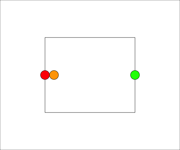
As example, a viewport with the x-scale going from 0 to 100 and the y-scale going from 0 to 10 (specified using xscale and yscale in viewport), the native unit can be used when locating a grob in that viewport on these scale values see example below
grid.newpage()# Erase/ clear the current device
# By default a root viewport is created
# and set as the current one

# Visualize the root viewport area
grid.draw(rectGrob())

# Create a new viewport
# default unit is set to "npc" so
# location of the viewport is normalized (0,1)
# with a xscale covering from 0 to 100
vp_1 <- viewport(name = "vp1",
                       width = 0.5, height = 0.5,
                       just = c("center", "center"),
                       xscale = c(0,100), yscale = c(0,10))
# Navigate into the viewport
pushViewport(vp_1)
# Visualize the vp_1 area
grid.draw(rectGrob())

# Draw some circles with location x, y , r (native)
grid.draw(circleGrob(x = unit(0, "native"), y = unit(5, "native"),
                     r = unit(5, "native"), gp = gpar(fill = "red")))
grid.draw(circleGrob(x = unit(10, "native"), y = unit(5, "native"),
                     r = unit(5, "native"), gp = gpar(fill = "orange")))
grid.draw(circleGrob(x = unit(100, "native"), y = unit(5, "native"),
                     r = unit(5, "native"), gp = gpar(fill = "green")))

popViewport()
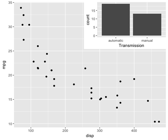
3. ggplot2 and the grid system: customize ggplot2 output
It is possible to use low-level functions in grid to customize/ manipulate the ggplot2 output. See the examples below.
grid.newpage()# Erase/ clear the current device

temp <- mtcars
temp[temp$am == 0,]$am <- "automatic"
temp[temp$am == 1,]$am <- "manual"
temp$am <- as.factor(temp$am)

basePlot <- ggplot(data = temp, mapping = aes(x = disp, y = mpg)) +
  geom_point()

grid.draw(ggplotGrob(basePlot))

vp_1 <- viewport(x = 1, y = 1,
                 just = c("right", "top"),
                 width = 0.5, height = 0.35)

pushViewport(vp_1)
miniPlot <- ggplot(data = temp, mapping = aes(x = am)) +
  geom_bar() + xlab("Transmission")
grid.draw(ggplotGrob(miniPlot))
popViewport()
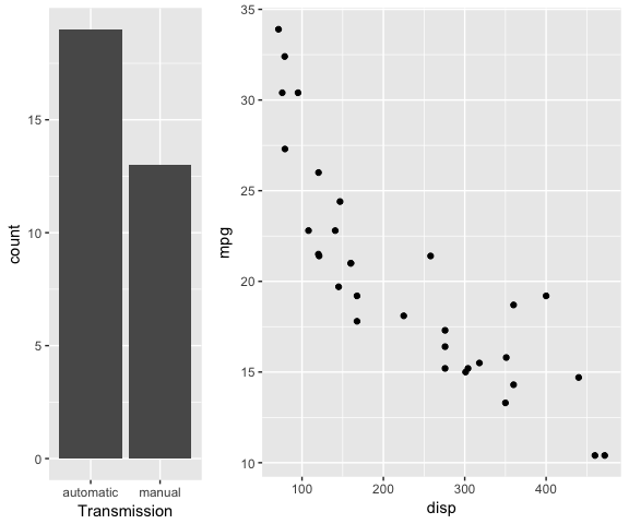
grid.newpage()# Erase/ clear the current device

vp_1 <- viewport(x = 0,
                 just = "left",
                 width = 1/3)

pushViewport(vp_1)
plot_r <- ggplot(data = temp, mapping = aes(x = am)) +
  geom_bar() + xlab("Transmission")
grid.draw(ggplotGrob(plot_r))
popViewport()

vp_2 <- viewport(x = 1/3,
                 just = "left",
                 width = 2/3)
pushViewport(vp_2)
plot_l <- ggplot(data = temp, mapping = aes(x = disp, y = mpg)) +
  geom_point()
grid.draw(ggplotGrob(plot_l))
popViewport()
4. Other packages
4.1 The gridExtra package
The gridExtra package provides useful extensions to the grid system focusing on higher-level functions to work with grid graphic objects. Interesting functions:
- arranging multiple grobs on a page [4],
- creating and manupilating layouts with graphical elements [5],
- adding tabular data alongside graphics [6].
5. Session Info
sessionInfo()
## R version 3.3.3 (2017-03-06)
## Platform: x86_64-apple-darwin13.4.0 (64-bit)
## Running under: macOS Sierra 10.12.6
##
## locale:
## [1] no_NO.UTF-8/no_NO.UTF-8/no_NO.UTF-8/C/no_NO.UTF-8/no_NO.UTF-8
##
## attached base packages:
## [1] grid      stats     graphics  grDevices utils     datasets  methods
## [8] base
##
## other attached packages:
## [1] ggplot2_2.2.1
##
## loaded via a namespace (and not attached):
##  [1] Rcpp_0.12.12     digest_0.6.12    rprojroot_1.2    plyr_1.8.4
##  [5] gtable_0.2.0     backports_1.1.0  magrittr_1.5     evaluate_0.10.1
##  [9] scales_0.5.0     rlang_0.1.2      stringi_1.1.5    lazyeval_0.2.0
## [13] rmarkdown_1.6    labeling_0.3     tools_3.3.3      stringr_1.2.0
## [17] munsell_0.4.3    yaml_2.1.14      colorspace_1.3-2 htmltools_0.3.6
## [21] knitr_1.17       tibble_1.3.4
6. References
[1] “The grid package” chapter in “Mastering Software Development in R” by Roger D. Peng, Sean Cross and Brooke Anderson, 2017
[2] Vignette “Introduction to grid” by Paul Murrell, April 2017
[3] Vignette “Working with grid viewports” by Paul Murrell, November 2016
[4] Vignette “Arranging multiple grobs on a page” by Baptiste Auguie, September 2017
[5] Vignette “(Unofficial) overview of gtable” by Baptiste Auguie, September 2017
[6] Vignette “Displaying tables as grid graphics” by Baptiste Auguie, September 2017
Interesting book:
- “R Graphics” 2nd Edition, by Paul Murrell, September 2015
Previous “Building Data Visualization Tools” blogs:
- Part 1: “Basic plotting with R and ggplot2”
- Part 2: “‘ggplot2’, essential concepts”
- Part 3: “Guidelines for good plots”
- Part 4: “How to work with maps”