Building Data Visualization Tools: New Graphical Elements in ‘ggplot2’

The content of this blog is based on examples/ notes/ experiments related to the material presented in the “Building Data Visualization Tools” module of the “Mastering Software Development in R” Specialization (Coursera) created by Johns Hopkins University [1] and supporting documentation on extending ggplot2 [2].

Required packages:

the ggplot2 package, the fundation for building new stat(s)/ geom(s)
the grid package, a catalog of building blocks for building new geom(s)
the gridExtra package, used for combined different plots.

# If a package is not locally installed
# install.packages("packageName")

library(ggplot2)
library(grid)
library(gridExtra)

Some Basic Concepts

Key elements in ggplot2 are geoms and stats, which allow to create interesting and rich data graphics and visualizations. The building new geoms or stats is the plotting equivalent of writing functions and it can be achieved using the extending mechanism/ framework provided by the ggplot2 package [2].

The building of a new geom/ stat feature follows a two step process:

use the ggplot2::ggproto() function to create a new class corresponding to your new feature,
- inheriting from the Geom or Stat class
implement the geom_* or stat_* function returning a graphic layer that can be added to a plot previously created using the ggplot() function.

All ggplot2 objects are created using the ggproto Object-Oriented System which allows the creation of mutable objects (for some more info about ggproto OOS see [2]).

A simple example of how to create a ggproto object can be found below …

# Create a ggproto object
A <- ggplot2::ggproto("_class" = "MyClass", "_inherit" = NULL,
                       x = 1,
                       inc = function(self){
                           self$x <- self$x + 1
                       })

# Check the structure of the object
str(A)
## Classes 'MyClass', 'ggproto' <ggproto object: Class MyClass>
##     inc: function
##     x: 1

# Visualize the value of x
A$x
## [1] 1

# Increment & visualize x
A$inc()
A$x
## [1] 2

How to create a new stat

All of the stat_* functions return a layer object, that is a combination of data, stat and geom with a potential position adjustment. The new Stat* class is a ggproto class and a Stat class (inheritance), overriding some specific methods (see ?Stat for more information).

Some examples from [2] …

# Stat used for the creation of a convex hull
# stat implementation
# (override) compute_group, called once per group
# (override) required_aes, aesthetics needed to render the geom

StatConvexHull <- ggproto("_class" = "StatConvexHull", "_inherit" = Stat,
                          compute_group = function(data, scales){
                              data[chull(data$x, data$y),, drop = FALSE]
                          },
                          required_aes = c("x", "y"))

# Implement the relevant stat_* function
# The function creates a new layer using the layer function
# note that the GeomPolygon geom is used with this stat

stat_convexHull <- function(geom = "polygon", data = NULL, mapping = NULL,
                            position = "identity", na.rm = F, inherit.aes = TRUE,
                            show.legend = NA, ...){

    layer(geom = geom, stat = StatConvexHull,
          data = data, mapping = mapping, position = position,
          inherit.aes = inherit.aes, show.legend = show.legend,
          params = list(na.rm = na.rm, ...))
}

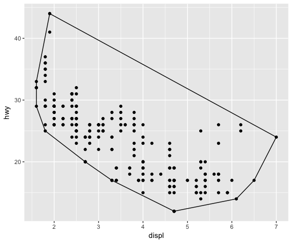
ggplot(data = mpg, mapping = aes(x = displ, y = hwy)) +
    geom_point() +
    stat_convexHull(fill = NA, colour = "black")

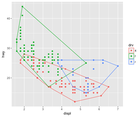
ggplot(data = mpg, mapping = aes(x = displ, y = hwy, colour = drv)) +
    geom_point() +
    stat_convexHull(fill = NA)

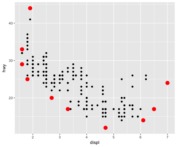
# Using a different geom (GeomPoint) with the new stat
ggplot(data = mpg, mapping = aes(x = displ, y = hwy)) +
    geom_point() +
    stat_convexHull(geom = "point", size = 4, colour = "red")

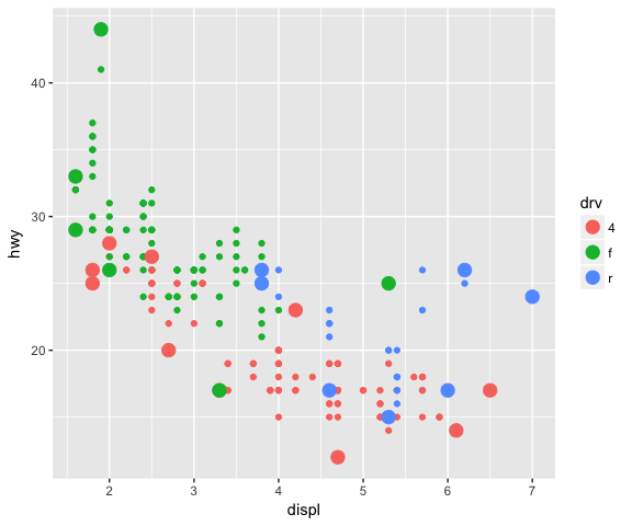
# Using a different geom (GeomPoint) with the new stat
ggplot(data = mpg, mapping = aes(x = displ, y = hwy, colour = drv)) +
    geom_point() +
    stat_convexHull(geom = "point", size = 4)

Another example from [2] …

# creation of a simple version of geom_smooth

StatLm <- ggproto("_class" = "StatLm", "_inherit" = Stat,

                  compute_group = function(data, scales, n = 100, formula = y ~ x){
                      rng <- range(data$x, na.rm = T)
                      grid <- data.frame(x = seq(rng[1], rng[2], length = n))

                      mod <- lm(formula, data = data)
                      grid$y <- predict(object = mod, newdata = grid)
                      grid
                  },

                  required_aes = c("x", "y")
                  )

# note that the GeomLine geom is used with this stat
stat_lm <- function(mapping = NULL, data = NULL, geom = "line",
                    position = "identity", na.rm = F, show.legend = NA,
                    inherit.aes = T, n = 50, formula = y ~ x, ...){

    layer(stat = StatLm, data = data, mapping = mapping, geom = geom, position = position,
          show.legend = show.legend, inherit.aes = inherit.aes,
          params = list(n = n, formula = formula, na.rm = na.rm, ...))

}

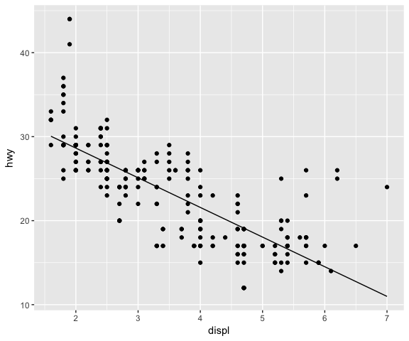
ggplot(data = mpg, mapping = aes(x = displ, y = hwy)) +
    geom_point() +
    stat_lm()

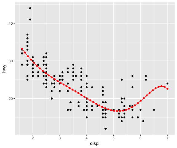
ggplot(data = mpg, mapping = aes(x = displ, y = hwy)) +
    geom_point() +
    stat_lm(formula = y ~ poly(x, 6), colour = "red")  +
    # Using a different geom (GeomPoint) with the new stat
    stat_lm(formula = y ~ poly(x, 6), geom = "point", n = 50, colour = "red")

Sometimes there are calculations that need to be performed only once for the dataset, not for each group. The setup_params function, defined in the Stat class, can be used for this purpose (see example below from [2]).

StatDensityCommon <- ggproto("_class" = "StatDensityCommon", "_inherit" = Stat,
                             required_aes = "x",
                             setup_params = function(data, params){
                                 # print("Running set_up....")
                                 if(!is.null(params$bandwidth)) return(params)

                                 xs <- split(data$x, data$group)
                                 bws <- vapply(xs, bw.nrd0, numeric(1))
                                 bw <- mean(bws)
                                 # message("Picking bandwidth of ", signif(bw, 3))

                                 params$bandwidth <- bw
                                 # print("End set_up....")
                                 params

                             },

                             compute_group = function(data, scales, bandwidth = 1){
                                 # print(paste("Running compute_group [", unique(data$group), "] ..."))
                                 # str(data)
                                 # print(bandwidth)
                                 d <- density(data$x,bandwidth)
                                 # print("End compute_group....")
                                 data.frame(x = d$x, y = d$y)
                             })

# note that the GeomLine geom is used with this stat
stat_densityCommon <- function(data = NULL, mapping = NULL, geom = "line",
                               position = "identity", na.rm = FALSE, show.legend = NA,
                               inherit.aes = T, bandwidth = NULL, ...){
    layer(geom = geom,  stat = StatDensityCommon, data = data, mapping = mapping, position = position,
          params = list(bandwidth = bandwidth, na.rm = na.rm, ...), inherit.aes = inherit.aes, show.legend = show.legend)
}

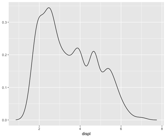
ggplot(data = mpg, mapping = aes(x = displ)) +
    stat_densityCommon(bandwidth = 0.25)

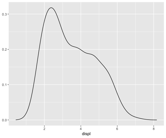
# Bandwidth is calculated from the data (once)
ggplot(data = mpg, mapping = aes(x = displ)) +
    stat_densityCommon()

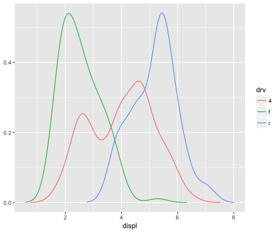
ggplot(data = mpg, mapping = aes(x = displ, colour = drv)) +
    stat_densityCommon()

Important aspects to consider: variable names and default aesthetics. If you want to make a stat usable with other geoms we need to be careful with the chosen names.

“If we want to make this stat usable with other geoms, we should return a variable called density instead of y. Then we can set up the default_aes to automatically map density to y, which allows the user to override it to use with different geoms.”

StatDensityCommon <- ggproto("StatDensityCommonE", Stat,
  required_aes = "x",
  default_aes = aes(y = ..density..),

  compute_group = function(data, scales, bandwidth = 1) {
    # print(paste("Running compute_group [", unique(data$group), "] ..."))
    d <- density(data$x, bw = bandwidth)
    # print(paste("x (range):", paste(range(d$x), collapse = " - "), "- bw:", bandwidth))
    data.frame(x = d$x, density = d$y)
  }  
)

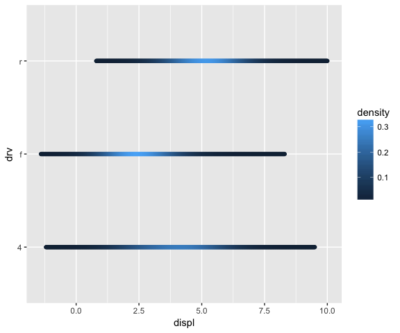
ggplot(mpg, aes(displ, drv, colour = ..density..)) +
  stat_densityCommon(bandwidth = 1, geom = "point")

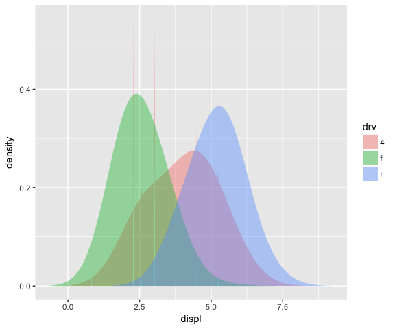
# Using this stat with the area geom doesn’t work quite right.
# The areas don’t stack on top of each other because each density
# is computed independently, and the estimated x-ranges don’t line up.
ggplot(mpg, aes(displ, fill = drv)) +
  stat_densityCommon(bandwidth = 0.75, geom = "area", position = "stack", alpha = 0.4)

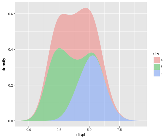
The setup_params function can be used to line up the x-ranges for the different groups. See example below from [2]…

StatDensityCommon <- ggproto("StatDensityCommonF", Stat,
  required_aes = "x",
  default_aes = aes(y = ..density..),

  setup_params = function(data, params){
      # print("Running set_up....")
      min <- min(data$x) - 3 * params$bandwidth
      max <- max(data$x) + 3 * params$bandwidth
      # print(paste("min:", min, "- max:", max, "- bw:", params$bandwidth))
      # print("End set_up....")
      list(
        bandwidth = params$bandwidth,
        min = min,
        max = max,
        na.rm = params$na.rm
      )
  },

  compute_group = function(data, scales, min, max, bandwidth = 1) {
    # print(paste("Running compute_group [", unique(data$group), "] ..."))
    d <- density(data$x, bw = bandwidth, from = min, to = max)
    # print(paste("x (range):", paste(range(d$x), collapse = " - "), "- bw:", bandwidth))
    # print("End compute_group....")
    data.frame(x = d$x, density = d$y)
  }  
)

ggplot(mpg, aes(displ, fill = drv)) +
  stat_densityCommon(bandwidth = 0.75, geom = "area", position = "stack", alpha = 0.4)

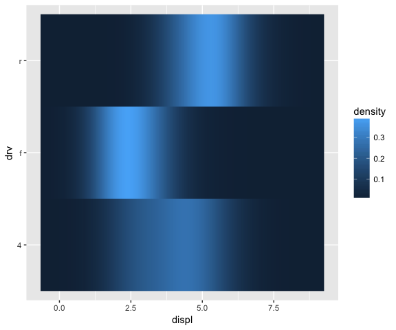
ggplot(mpg, aes(displ, drv, fill = ..density..)) +
  stat_densityCommon(bandwidth = 0.75, geom = "raster")

How to create a new geom

All of the geom_* functions return a layer that contains a Geom* object (instance of the Geom* class), responsible for rendering the data in the plot. The Geom* class is a ggproto class and a Geom class (inheritance), overriding some specific methods/ fields (see ?Geom for more information).

Specific methods/ fields are

required_aes, a character vector of needed aesthetics
default_aes, a list of default values for aesthetics
draw_key, a function used to draw key in the legend
either draw_panel or draw_group function returning a grid grob to be plotted

The draw_panel function can be used when data is plot by panels and, each row in data represents a graphic element in a panel. See examples below from [2]…

GeomMyPoint <- ggproto("_class" = "GeomMyPoint", Geom,
                       required_aes = c("x", "y"),
                       default_aes = aes(shape = 1),
                       draw_key = draw_key_point,
                       draw_panel = function(data, panel_scales, coord){
                           # Transform the data first
                           coords <- coord$transform(data, panel_scales)

                           # Construct & return a grid object
                           pointsGrob(x = coords$x,
                                      y = coords$y,
                                      pch = coords$shape)
                       })

geom_mypoint <- function(mapping = NULL, data = NULL, stat = "identity",
                         position = "identity", na.rm = FALSE,
                         show.legend = NA, inherit.aes = TRUE, ...) {
        ggplot2::layer(
                geom = GeomMyPoint, mapping = mapping,  
                data = data, stat = stat, position = position,
                show.legend = show.legend, inherit.aes = inherit.aes,
                params = list(na.rm = na.rm, ...)
        )
}

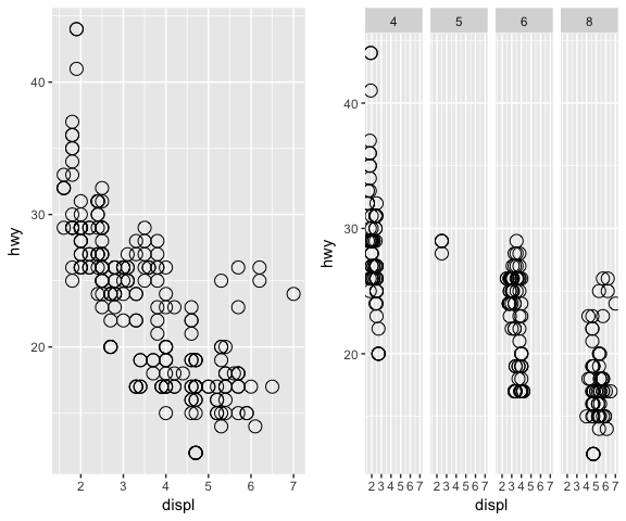
base_plot <- ggplot(data = mpg, mapping= aes(x = displ, y = hwy))

one_panel <- base_plot  + geom_mypoint()

multi_panels_by_cyl <- base_plot  +
    geom_mypoint() +
    facet_grid(. ~ cyl)

grid.arrange(one_panel, multi_panels_by_cyl, nrow = 1)

The draw_group function can be used when the data is plot by groups and, one graphic element must be plot per each group. See example below (inspired by [2]) used to create a Geom that is plotting the convex hull of the provided polygon with its centroid …

GeomCentroidPolygon <- ggproto("GeomCentroidPolygon", Geom,

                               required_aes = c("x", "y"),

                               default_aes = aes(colour = "black", fill = "grey70", size = 0.5,
                                                 linetype = 1, alpha = 1),

                               draw_key = draw_key_polygon,

                               draw_group = function(data, panel_scales,coord){
                                 n <- nrow(data)
                                 if(n <= 2) return(grid::nullGrob())

                                 coords <- coord$transform(data, panel_scales)
                                     first_row <- coords[1, , drop = FALSE]

                                 centroid_x <- mean(coords$x, na.rm = T)
                                 centroid_y <- mean(coords$y, na.rm = T)

                                 poly_elem <- grid::polygonGrob(name = "polygonChull",
                                   x = coords$x, y = coords$y,
                                   default.units = "native",
                                   gp = grid::gpar(
                                     col = first_row$colour,
                                     fill = scales::alpha(first_row$fill, first_row$alpha),
                                     lwd = first_row$size * .pt,
                                     lty = first_row$linetype
                                   )
                                 )

                                 centroid_elem <- grid::pointsGrob(name = "centroid",
                                                                   x = centroid_x, y = centroid_y,
                                                                   gp = grid::gpar(col = first_row$colour),
                                                                   pch = 4)

                                 gTree(children = gList(poly_elem, centroid_elem))

                               })

geom_centroid_polygon <- function(mapping = NULL, data = NULL, stat = "convexHull",
                                position = "identity", na.rm = FALSE, show.legend = NA,
                                inherit.aes = TRUE, ...) {
  layer(
    geom = GeomCentroidPolygon, mapping = mapping, data = data, stat = stat,
    position = position, show.legend = show.legend, inherit.aes = inherit.aes,
    params = list(na.rm = na.rm, ...)
  )
}

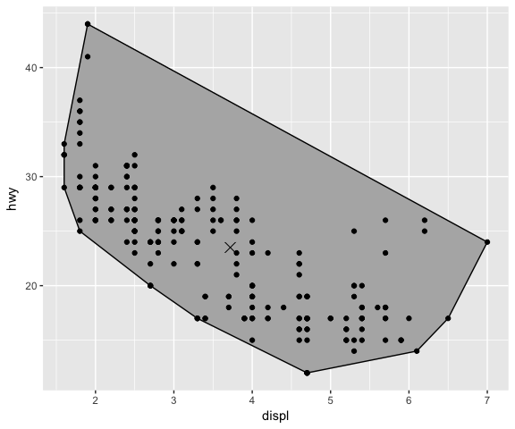
ggplot(mpg, aes(displ, hwy)) +
  geom_centroid_polygon()+
  geom_point()

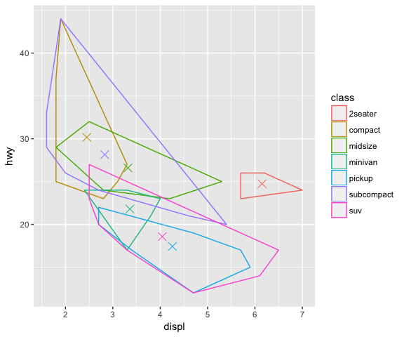
ggplot(mpg, aes(displ, hwy, colour = class)) +
  geom_centroid_polygon(fill = NA)

Summary

Building new graphical elements, stat(s) or geom(s),can be useful if a new new graphical element is needed or to simplify a complex graphical task/ process that must be used repeatedly in many plots. The building of the new graphical element is done using the extending mechanism provided by ggplot2 [2]. More examples of ggplot2 extension can be found at [3].

References

[1] “Building New Graphical Elements” chapter in “Mastering Software Development in R” by Peng, Cross and Anderson, 2017
[2] Article “Extending ggplot2”
[3] Some examples of ggplot2-extensions

Interesting book:

“R Graphics” 2nd Edition, by Paul Murrell, September 2015

Previous “Building Data Visualization Tools” blogs:

Part 1: “Basic plotting with R and ggplot2”
Part 2: “‘ggplot2’, essential concepts”
Part 3: “Guidelines for good plots”
Part 4: “How to work with maps”
Part 5: “Customise ggplot2 output with grid”

Session Info

sessionInfo()
## R version 3.3.3 (2017-03-06)
## Platform: x86_64-apple-darwin13.4.0 (64-bit)
## Running under: macOS  10.13
##
## locale:
## [1] no_NO.UTF-8/no_NO.UTF-8/no_NO.UTF-8/C/no_NO.UTF-8/no_NO.UTF-8
##
## attached base packages:
## [1] grid      stats     graphics  grDevices utils     datasets  methods  
## [8] base     
##
## other attached packages:
## [1] gridExtra_2.3 ggplot2_2.2.1
##
## loaded via a namespace (and not attached):
##  [1] Rcpp_0.12.12     digest_0.6.12    rprojroot_1.2    plyr_1.8.4      
##  [5] gtable_0.2.0     backports_1.1.0  magrittr_1.5     evaluate_0.10.1
##  [9] scales_0.5.0     rlang_0.1.2      stringi_1.1.5    reshape2_1.4.2  
## [13] lazyeval_0.2.0   rmarkdown_1.6    labeling_0.3     tools_3.3.3     
## [17] stringr_1.2.0    munsell_0.4.3    yaml_2.1.14      colorspace_1.3-2
## [21] htmltools_0.3.6  knitr_1.17       tibble_1.3.4

Discovering the new Digital world